1. Introduction
Land-cover maps provide information for natural resource and ecosystem service management, conservation planning, urban planning, agricultural monitoring, and the assessment of long-term land change. The automated classification of land cover from satellite imagery is a challenging task due to spectral mixing, intra-class spectral variability, and low spectral contrast among classes. Hyperspectral, or imaging spectroscopy, data consist of hundreds of spectral bands, and capture more spectral detail and variability relative to conventional multispectral sensors used for mapping land cover. Terrestrial hyperspectral applications have shown success in mapping composition, physiology, and biochemistry of vegetation, ecosystem disturbance, and built-up environments [
1]. The analysis of hyperspectral data presents issues in classification, due to large data volumes, and increased spectral variability as recorded by hundreds of correlated bands [
2]. Additionally, the classification task becomes more difficult when presented with the larger spatial extents and temporally detailed data collected by spaceborne hyperspectral sensors with repeat measurements.
A traditional classification method for hyperspectral imagery involves Multiple Endmember Spectral Mixture Analysis (MESMA), which consists of unmixing image spectra with pure spectral profiles (endmembers), and assigning the class through endmembers selected in the unmixing solution [
3]. This family of methods typically requires regionally specific libraries of pure spectral profiles that are from field spectra, synthetically generated, or selected from large libraries of image spectra [
4]. This type of classification is the most closed form solution available currently, analytically processing an exhaustive combination of endmembers that most closely match the data to be classified [
3]. Further, MESMA assumes linear mixing, which is often violated by the interaction of photons with components within an individual pixel and from nearby pixels.
Machine learning is an alternative domain of classification techniques that can accurately distinguish land cover in hyperspectral and multi-seasonal imagery [
5]. In contrast to MESMA, these classifiers can learn non-linear decision spaces and do not require training data optimization steps to select spectrally pure endmembers. There are many different varieties of machine learning algorithms implemented on different platforms. Picking the classifier to analyze a dataset at times falls to the user’s familiarity with the computational platform and/or algorithm for a specific field. Random Forests (RF) and Support Vector Machines (SVM) are widely adopted machine learning classifiers in the remote sensing community [
6,
7]. These algorithms have provided robust results across many platforms and datasets, surpassing many other families and implementations of classifiers [
8].
Convolutional Neural Network (CNN) is a leading machine learning classifier for image recognition tasks that use 2-dimensional (2-D) image data [
9,
10], such as identifying faces in photographs of people. Applications of CNN have extended into the classification of other contiguous data types, like speech recognition utilizing 1-dimensional (1-D) data [
11]. In remote sensing, there have been several recent applications of CNNs and other similar “deep” network topologies [
12,
13,
14,
15,
16,
17,
18]. The form in which CNNs are applied to remote sensing data can vary significantly depending on the data available, as there is no universal deep network classification architecture. The application of a CNN to classify land cover from 2-D visual images has been performed with good results in their respective applications. For example, Kussel et al. [
15] achieved a 95% overall accuracy with land-cover classification and Li et al. [
19] had a 96% correct detection of plants within a scene. In some applications, segmentation and previously learned features can be transferred and leveraged as part of the CNN classification task [
12,
20,
21,
22]. The method within [
18,
23,
24] applies down-selected spectra to a 2-D CNN architecture, thereby mainly exploiting the spatial extent of the data. The spectral dimension is reduced because large number of features present with hyperspectral imagery typically poses a problem for some classifiers, and many studies use dimensionality reduction (DR) to aid in the classification process [
13,
18,
23,
24,
25,
26]. In [
23,
24,
25] the spectral dimension was reduced, for example by applying principal component analysis [
23,
24], comparing salient band vectors in a manifold ranking space to consider hyperspectral data structure [
25], or clustering similar bands and extracting features [
26]. All these methods reduce the number of spectral bands before subjecting the data to the classifier. The method provided in [
6] pre-calculates features based on physical and chemical composition. All these DR methods have shown an increase in classification accuracy as compared to using the full hyperspectral data. In contrast, some studies have shown increased classification accuracy when utilizing the full spectra, invalidating the need for complex DR preprocessing. For example, the work done in [
13] shows the comparison between a 3-dimensional (3-D) CNN, which utilizes the full spectral dimension, and other methods that do not utilize the full spectral dimension. The 3-D CNN spanning the full spectral dimension increased accuracy by up to 3%. In this case, the CNN classifier determines what are the distinctive features from the initial data, without a DR pre-processing step. As another example, Hu et al. [
17] utilized single-season hyperspectral data and 1-D CNN across the full spectral dimension to classify land cover with 90 to 93% overall accuracy, and CNN outperformed SVM by 1 to 3%. A distinction between the extraction of key spectra by using DR and spectral feature generation from the CNN is that the CNN approach extracts features based on spectral characteristics directly driven from reducing classification error. This makes CNN a promising method for the exploitation of the distinctive aspects of the spectral dimension of the data and warrants further investigation with hyperspectral land-cover mapping applications at various spatial and temporal scales.
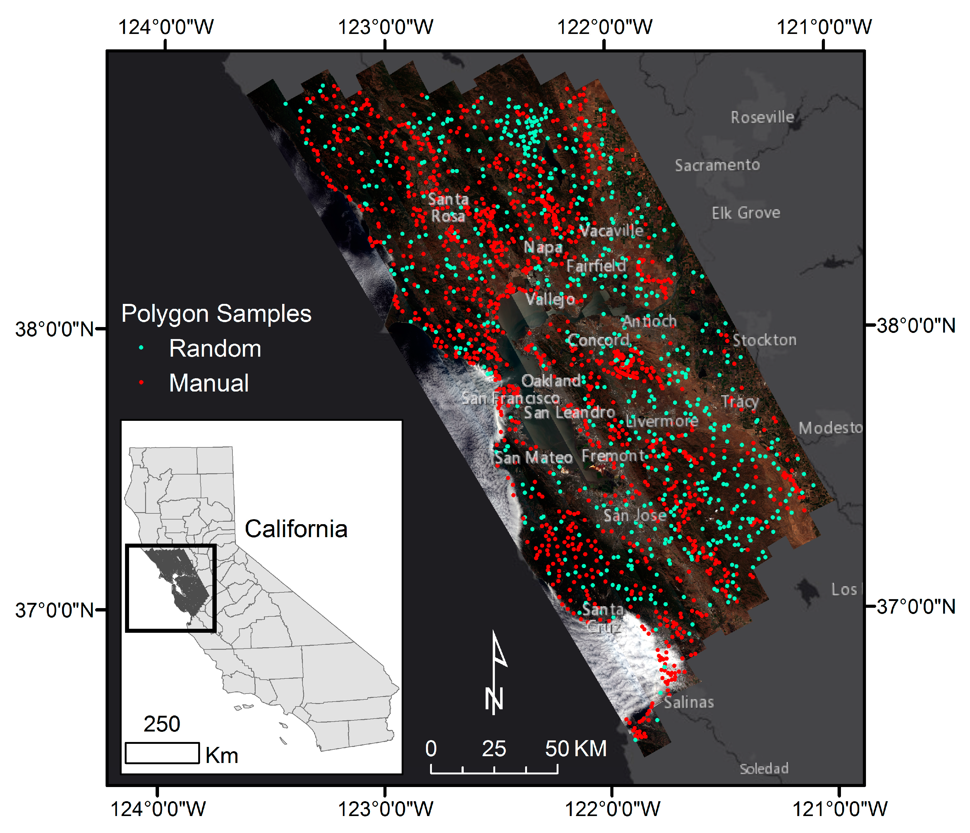
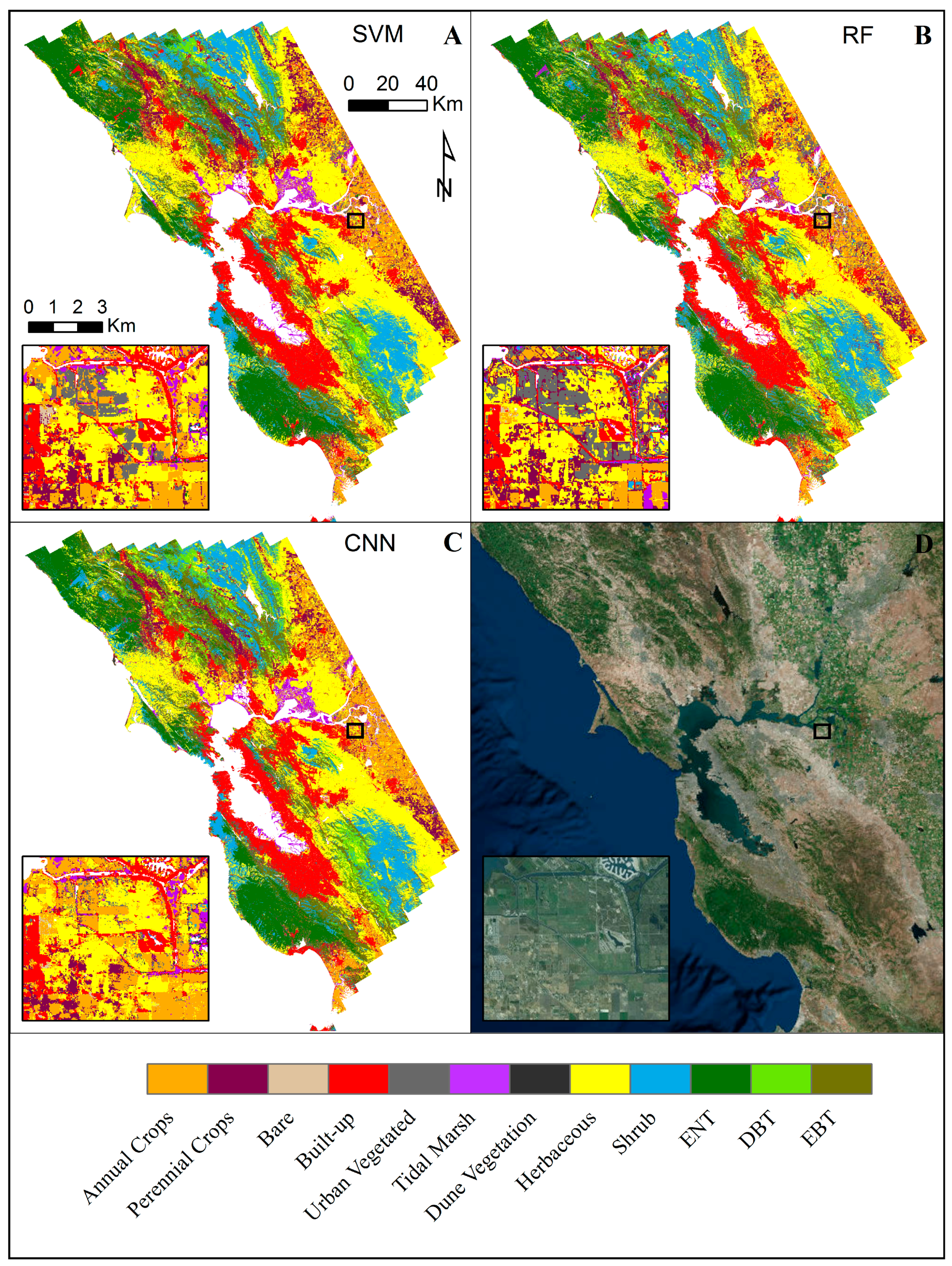
A broad goal of this study is to assess the accuracy of a 1-D CNN for classifying land cover from multi-seasonal hyperspectral imagery. Accuracy from this CNN is compared to those from the two leading machine learning classification methods in remote sensing, RF and SVM. These methods were utilized as a control group due to their high accuracy rates, high prevalence within the field and the robust libraries available for their implementation. In order to support applications based on spaceborne hyperspectral imagery, our analyses were performed with simulated Hyperspectral Infrared Imager (HyspIRI) imagery, a satellite mission currently being considered by NASA. Our analyses are regional in scale, covering the San Francisco Bay Area, California, and land-cover classes followed the global Land-Cover Classification System (LCCS) [
27].
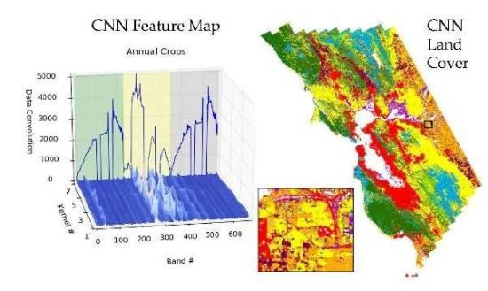
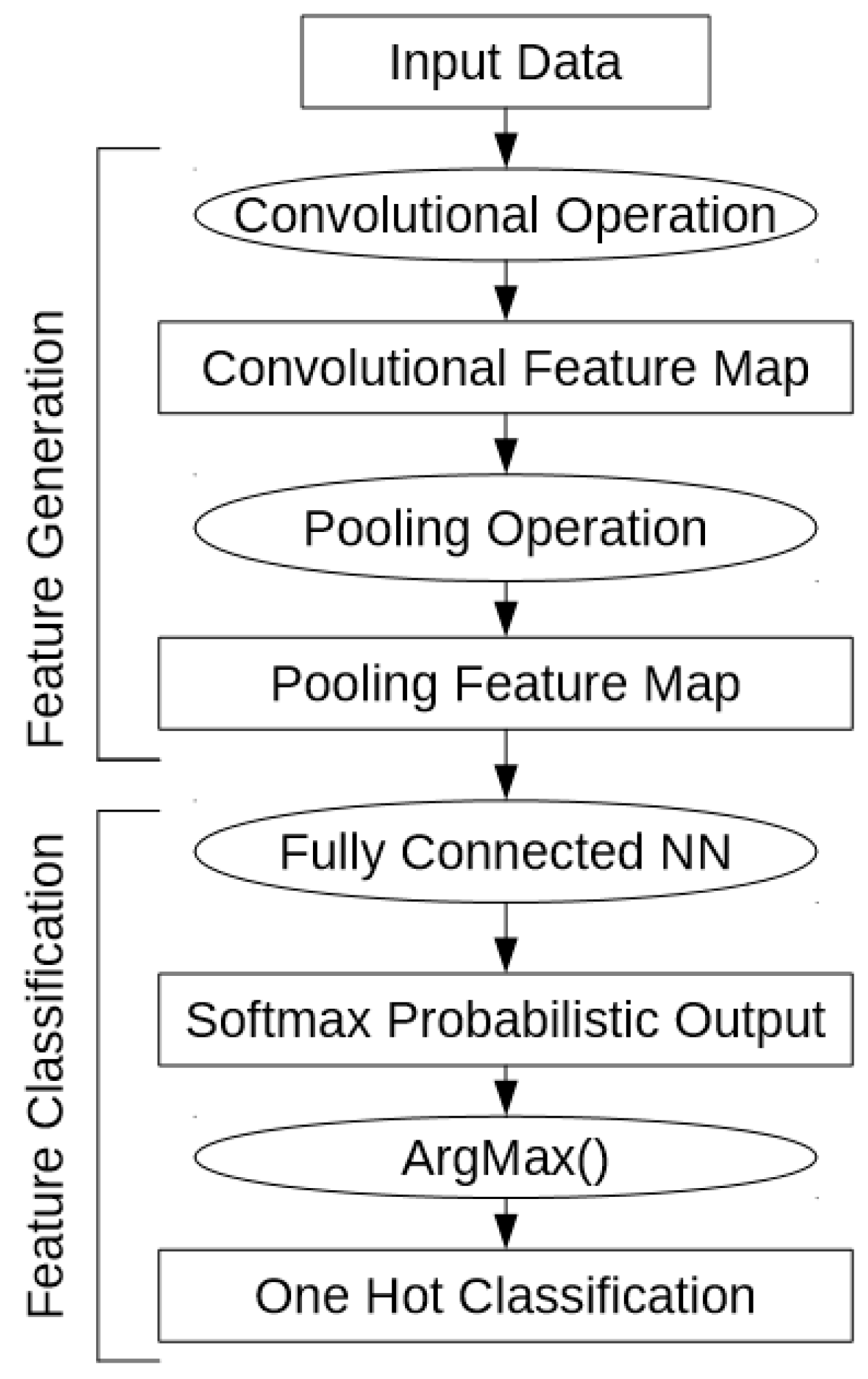
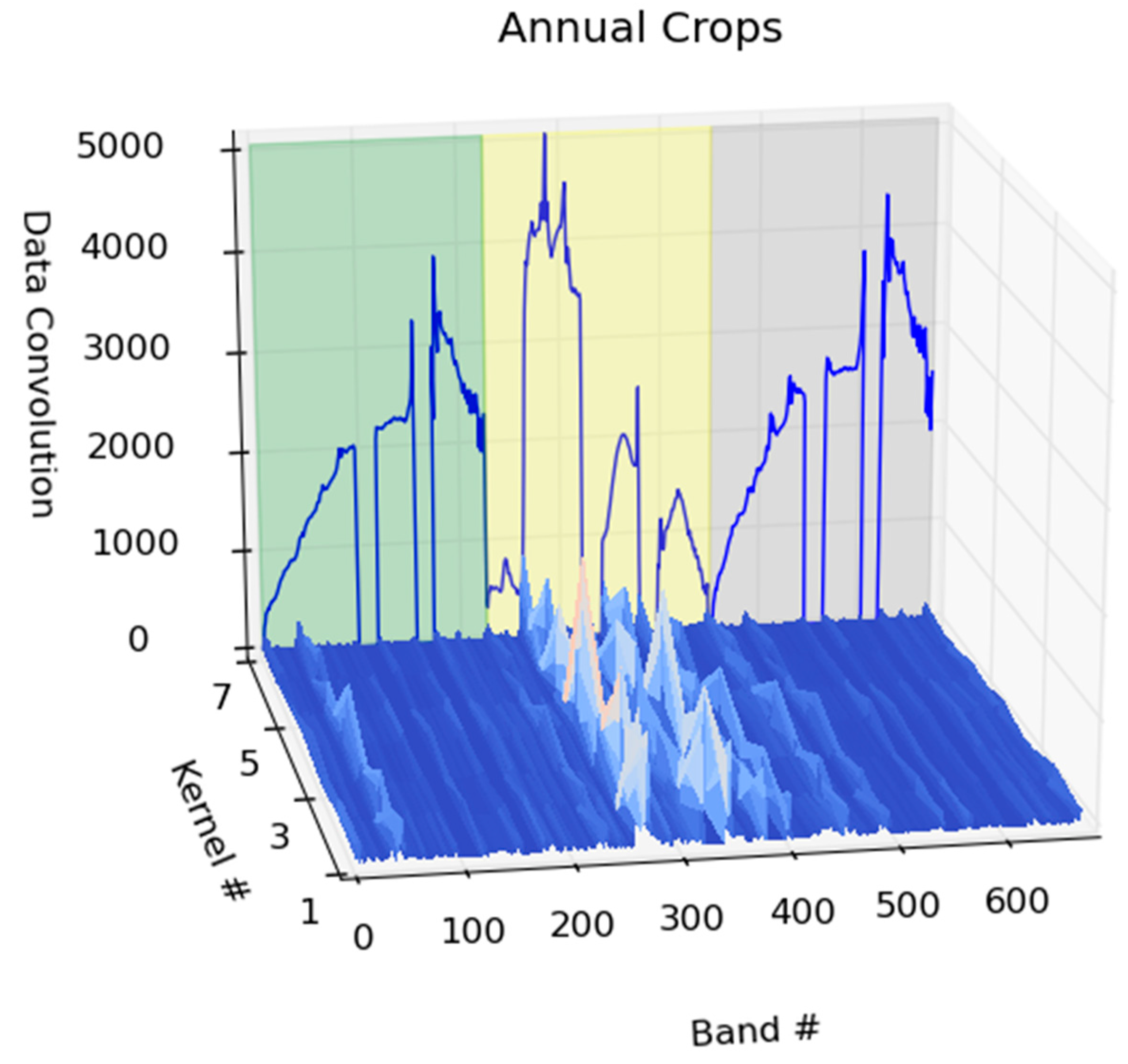
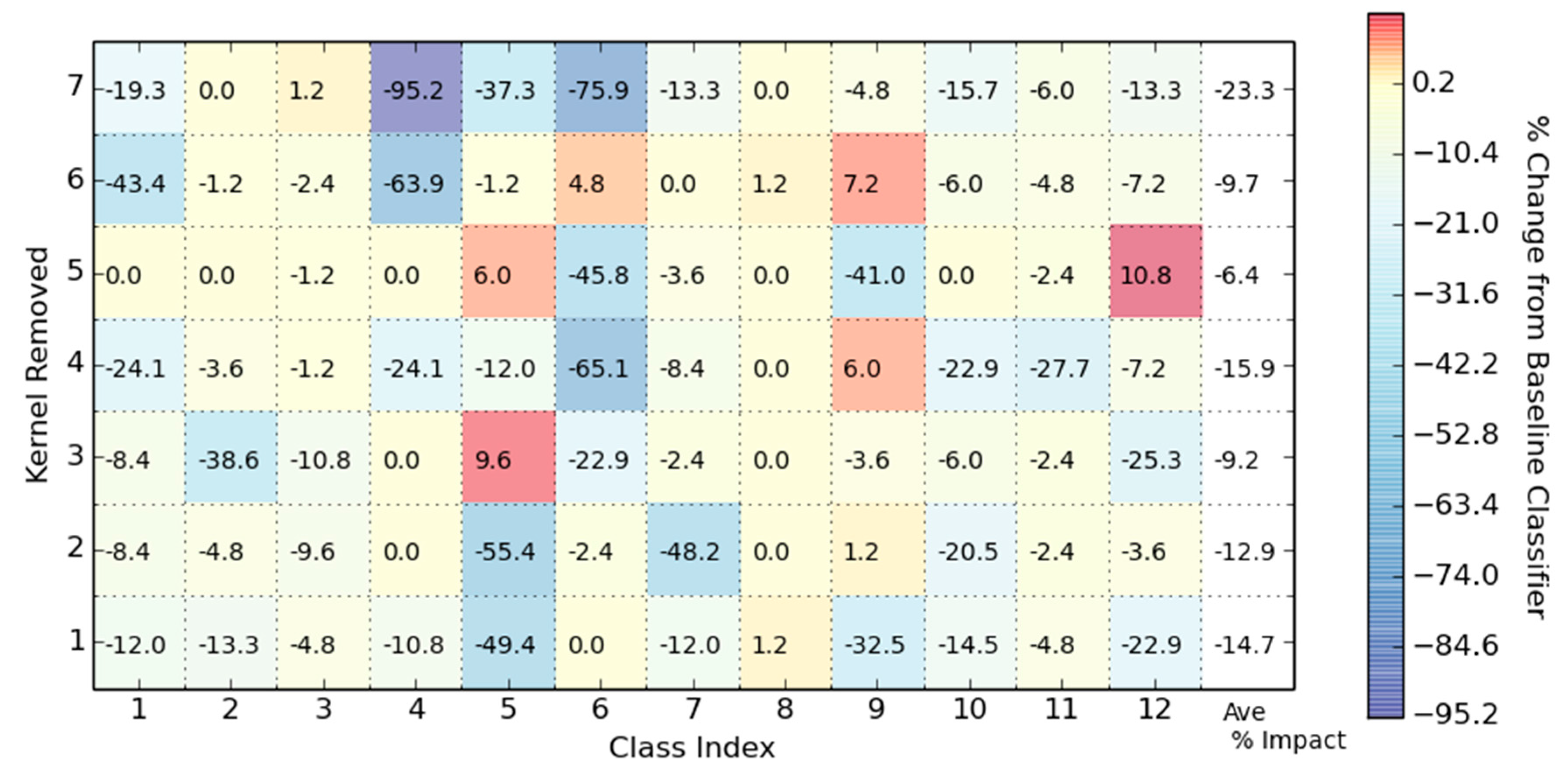
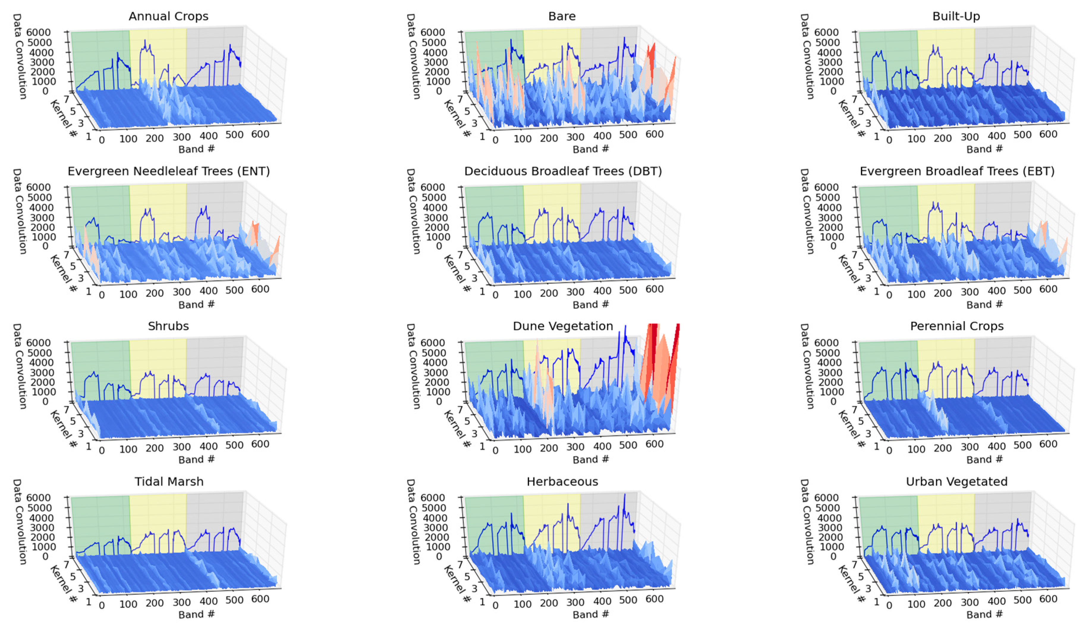
A CNN architecture requires the data to be in a contiguous format as convolutional layers of the network distinguish, or filter, local features or patterns from neighboring regions throughout the data. The neural network then performs the subsequent classification based on these learned features. A potentially useful feature of CNN architectures is that the inner resulting data products, such as properties of convolutional filters, can provide some insight into what the classifier has learned to make its classification. The inner data products of CNN architectures as applied to 1-D hyperspectral data have not been discussed in the literature. Thus, another goal of this study is to show how the inner data products of CNN can provide insight into the classification task and the features extracted from the spectra through the training of the network. With the analysis of feature maps that the convolutional layer of this network creates, local regions within the spectral dimension of the data that are excited by the convolutional layer of the network can be shown to have an impact on the classification accuracy. The importance of these learned features can be then traced back to how important they are to the classification task, by zeroing them from the network and re-computing the accuracy. Additional processing of the feature maps extracted from the CNN enables an illustrative visual that reveals which spectral areas assist in separating the classes. By standardizing, scaling and capturing only the magnitude of the convolutional kernel feature maps, the spectral-temporal band importance can be visually explored.


