A porous slider with velocity slip

It is well known that the drag is greatly reduced if a moving body is levitated by a layer of air. Examples of this include air hockey and air-cushioned vehicles. Very often, a fluid is injected uniformly from the porous bottom of a moving body, which we term a porous slider. The first fluid dynamics analysis of the lift and drag of a porous slider was by Wang (1974), who studied a laterally moving circular disc that is levitated by bottom fluid injection. The strip slider was studied by Skalak and Wang (1975) and the elliptic slider by Watson et al (1978). In all the cases, the solutions are exact similarity solutions of the Navier–Stokes equations. For more recent variations, see the works of Hinch and Lemaitre (1994), Cox (2002) and Khan et al (2011).

All the above-cited references used the no-slip condition on both the slider and the immobile ground. However, the velocity slip should be included in the following cases. (i) The fluid could be a rarefied gas, where there exists a slip flow regime (Sharipov and Seleznev 1998). (ii) The 'ground' could be rough such that an equivalent slip is present (Wang 2003). (iii) The solid surface could be coated with a substance that resists adhesion (e.g. Teflon or a lubricant). (iv) The porous bottom of the slider, from where the fluid is injected, would not have zero mean tangential velocity (Ng and Wang 2009). (v) Slip is especially important for super-hydrophobic surfaces (Choi et al 2006).

The aim of this paper is to study the effect of slip on the performance of the porous slider. Instead of the no-slip condition, we shall use the partial slip condition first proposed by Navier (1827):

$$\begin{equation} u = N\tau . \end{equation} \tag{ 1 }$$

Here the tangential velocity u is proportional to the shear stress τ , and N is the proportional slip coefficient. We assume that the slider-to-ground gap width is much smaller than the slider's lateral dimension, such that end effects can be ignored. Our solutions are also exact similarity solutions to the Navier–Stokes equations. We shall study both the strip slider and the circular slider.

Consider a long slider as shown in figure 1(a), where its length in the y-direction is much larger than its width in the x-direction. Both the length and the width are much greater than the gap width d. The slider is levitated by fluid injection from its bottom with velocity W and slides with velocity components U and V as shown. We fix our axes on the slider such that the slider is still and the ground moves laterally (i.e. with velocities U, V in the positive x- and y-direction). The steady, constant property Navier–Stokes equations are

$$\begin{equation} uu_x + \upsilon u_y + wu_z = - p_x /\rho + \nu (u_{xx} + u_{yy} + u_{zz} ), \end{equation} \tag{ 2 }$$

$$\begin{equation} u\upsilon _x + \upsilon \upsilon _y + w\upsilon _z = - p_y /\rho + \nu (\upsilon _{xx} + \upsilon _{yy} + \upsilon _{zz} ), \end{equation} \tag{ 3 }$$

$$\begin{equation} uw_x + \upsilon w_y + ww_z = - p_z /\rho + \nu (w_{xx} + w_{yy} + w_{zz} ), \end{equation} \tag{ 4 }$$

Zoom In Zoom Out Reset image size

where (u,υ ,w) are the velocity components in the Cartesian (x,y,z) coordinates, p is the pressure, ρ is the density and ν is the kinematic viscosity. The continuity equation is

$$\begin{equation} u_x + \upsilon _y + w_z = 0. \end{equation} \tag{ 5 }$$

Due to symmetry, all variables are independent of the longitudinal direction y. Skalak and Wang (1975) used the following similarity transform:

$$\begin{equation} u = \frac{W}{d}xh'(\eta ) + Uf(\eta ), \end{equation} \tag{ 6 }$$

$$\begin{equation} \upsilon = Vg(\eta ), \end{equation} \tag{ 7 }$$

$$\begin{equation} w = - Wh(\eta ), \end{equation} \tag{ 8 }$$

where η = z/d. Equations (2)–(5) reduce to the nonlinear ordinary differential equations

$$\begin{equation} h'h'' - hh'\,'' = \frac{1}{R}h''\,'', \end{equation} \tag{ 9 }$$

$$\begin{equation} h'f - hf' = \frac{1}{R}f'', \end{equation} \tag{ 10 }$$

$$\begin{equation} - hg' = \frac{1}{R}g''. \end{equation} \tag{ 11 }$$

Here R = Wd/ν is the cross-flow Reynolds number. Using Navier's slip conditions, the boundary conditions are that on z = 0:

$$\begin{equation} u - U = N_1 \mu \,u_z ,\quad \upsilon - V = N_1 \mu \,\upsilon _z ,\quad w = 0 \end{equation} \tag{ 12 }$$

and that on z = d:

$$\begin{equation} u = - N_2 \mu u_z ,\quad \upsilon = - N_2 \mu \upsilon _z ,\quad w = - W. \end{equation} \tag{ 13 }$$

Here N₁ and N₂ are different slip coefficients and μ = ρ ν is the viscosity. Equations (12) and (13) give

$$\begin{equation} h'(0) = \lambda _1 h''(0),\quad h(0) = 0, \end{equation} \tag{ 14 }$$

$$\begin{equation} h'(1) = - \lambda _2 h''(1),\quad h(1) = 1, \end{equation} \tag{ 15 }$$

$$\begin{equation} f(0) - 1 = \lambda _1 f'(0),\quad f(1) = - \lambda _2 f'(1), \end{equation} \tag{ 16 }$$

$$\begin{equation} g(0) - 1 = \lambda _1 g'(0),\,\,\,\,\,\,g(1) = - \lambda _2 g'(1), \end{equation} \tag{ 17 }$$

where λ₁ = N₁ μ /d, λ₂ = N₂μ/d are normalized slip factors. Equations (9)–(11) and (14)–(17) are to be solved.

Of interest are the forces on the slider. Using equations (2)–(4) the pressure is

$$\begin{equation} - \frac{p}{\rho } = K\frac{{W^2 x^2 }}{{2d}} + \frac{1}{2}w^2 - \nu w_z + C, \end{equation} \tag{ 18 }$$

where K, C are constants and

$$\begin{equation} K = (h')^2 - hh'' - \frac{1}{R}h'\,'' = [h'(0)]^2 - \frac{1}{R}h'\,''(0). \end{equation} \tag{ 19 }$$

If the slider has width 2l and the ambient pressure is p₀ , then equation (18) gives

$$\begin{equation} p - p_0 = - \rho \frac{{KW^2 (x^2 - l^2 )}}{{2d^2 }}. \end{equation} \tag{ 20 }$$

The lift per depth of the slider is then

$$\begin{equation} L = \int_{ - l}^l {(p - p_0 )\,{\rm{d}}x} = \frac{{2\rho W^2 l^3 }}{{3d^2 }}K. \end{equation} \tag{ 21 }$$

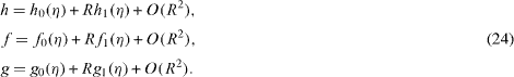
Thus K is the lift normalized by 2ρ W² l³ /(3d² ) . The drag per depth in the x-direction is

$$\begin{equation} D_x = - \int_{ - l}^l {\mu \frac{{\partial u}}{{\partial z}}} \left| {_{z = d} } \right.\,{\rm{d}}x = - \frac{{2\mu lU}}{d}f'(1). \end{equation} \tag{ 22 }$$

The drag in the x-direction normalized by 2μ lU/d is -f'(1) . Similarly the drag per depth in the y-direction is

$$\begin{equation} D_y = - \int_{ - l}^l {\mu \frac{{\partial \upsilon }}{{\partial z}}} \left| {_{z = d} } \right.\,{\rm{d}}x = - \frac{{2\mu lV}}{d}g'(1). \end{equation} \tag{ 23 }$$

The normalized drag is -g'(1) .

Some analytic approximations can be obtained for small or large Reynolds numbers. If R ≪ 1, we expand

$$\begin{eqnarray} &&h = h_0 (\eta ) + Rh_1 (\eta ) + O(R^2 ),\nonumber\\ &&f = f_0 (\eta ) + Rf_1 (\eta ) + O(R^2 ),\\ &&g = g_0 (\eta ) + Rg_1 (\eta ) + O(R^2 ).\nonumber \end{eqnarray} \tag{ 24 }$$

Equations (9)–(11) and (14)–(17) become successively

$$\begin{equation} \fl h_0 ''\,'' = 0,\quad h_0 (0) = 0,\quad h_0' (0) = \lambda _1 h_0 '' (0),\quad h_0 (1) = 1,\quad h_0' (1) = - \lambda _2 h_0 '' (1), \end{equation} \tag{ 25 }$$

$$\begin{equation} f_0 '' = 0,\quad f_0 (0) - 1 = \lambda _1 f_0' (0),\quad f_0 (1) = - \lambda _2 f_0' (1), \end{equation} \tag{ 26 }$$

$$\begin{equation} g_0 '' = 0,\quad g_0 (0) - 1 = \lambda _1 g_0' (0),\quad g_0 (1) = - \lambda _2 g_0' (1), \end{equation} \tag{ 27 }$$

$$\begin{eqnarray} &&h_1 ''\,'' = h_0' h_0 '' - h_0 h_0'\,'', \nonumber\\ &&h_1 (0) = 0,\quad h_1' (0) = \lambda _1 h_1 '' (0),\quad h_1 (1) = 0,\quad h_1' (1) = - \lambda _2 h_1 '' (1), \end{eqnarray} \noindent \tag{ 28 }$$

$$\begin{equation} f_1 '' = f_0 h_0' - h_0 f_0' ,\quad f_1 (0) = \lambda _1 f_1' (0),\quad f_1 (1) = - \lambda _2 f_1' (1), \end{equation} \tag{ 29 }$$

$$\begin{equation} g_1 '' = - h_0 g_0' ,\quad g_1 (0) = \lambda _1 g_1' (0),\quad g_1 (1) = - \lambda _2 g_1' (1). \end{equation} \tag{ 30 }$$

The solutions are found using a symbolic computer program:

$$\begin{equation} h_0 = \frac{{\eta [ - 2(1 + \lambda _1 + \lambda _2 )\eta ^2 + 3(1 + 2\lambda _2 )(\eta + 2\lambda _1 )]}}{{1 + 4(\lambda _1 + \lambda _2 ) + 12\lambda _1 \lambda _2 }}, \end{equation} \tag{ 31 }$$

$$\begin{equation} f_0 = g_0 = \frac{{ - \eta + 1 + \lambda _2 }}{{1 + \lambda _1 + \lambda _2 }}, \end{equation} \noindent \tag{ 32 }$$

$$\begin{eqnarray} &&\fl h_1 = \frac{1}{{70[1 + 4\lambda _2 + 4\lambda _1 (1 + 3\lambda _2 )]^3 }}\eta \left\{ {4\eta ^6 (1 + \lambda _1 + \lambda _2 )^2 [1 + 4\lambda _2 + 4\lambda _1 (1 + 3\lambda _2 )]} \right.\nonumber\\ &&- 14\eta ^5 (1 + 2\lambda _2 )[1 + 5\lambda _2 + 4\lambda _2^2 + 4\lambda _1^2 (1 + 3\lambda _2 ) + \lambda _1 (5 + 20\lambda _2 + 12\lambda _2^2 )]\nonumber\\ &&+ 21\eta ^3 (\eta + 5\lambda _1 )(1 + 2\lambda _2 )^2 [1 + 4\lambda _2 + 4\lambda _1 (1 + 3\lambda _2 )]\nonumber\\ &&- 3\eta ^2 [9 + 90\lambda _2 + 272\lambda _2^2 + 296\lambda _2^3 + 16\lambda _1^3 (1 + 7\lambda _2 ) + 2\lambda _1^2 (101 + 808\lambda _2\nonumber\\ &&+ 1932\lambda _2^2 + 1680\lambda _2^3 ) + \lambda _1 (90 + 810\lambda _2 + 2176\lambda _2^2 + 2072\lambda _2^3 )]\nonumber\\ &&+ (\eta + 2\lambda _1 )[16\lambda _1^2 (1 + 9\lambda _2 ) + 4(4 + 44\lambda _2 + 139\lambda _2^2 + 162\lambda _2^3 )\nonumber\\ &&+ \lambda _1 (95 + 950\lambda _2 + 2556\lambda _2^2 + 2520\lambda _2^3 )\left. ] \right\}, \end{eqnarray} \tag{ 33 }$$

$$\begin{eqnarray} &&\fl f_1 = \frac{1}{{20(1 + \lambda _1 + \lambda _2 )^2 [1 + 4\lambda _2 + 4\lambda _1 (1 + 3\lambda _2 )]}}\left\{ { - 4\eta ^5 (1 + \lambda _1 + \lambda _2 )^2 } \right.\nonumber\\ &&+ 5\eta ^4 [3 + 9\lambda _2 + 8\lambda _2^2 + 2\lambda _2^3 + 2\lambda _1^2 (1 + \lambda _2 ) + \lambda _1 (5 + 10\lambda _2 + 4\lambda _2^2 0] \nonumber\\ &&- 20\eta ^2 (\eta + 3\lambda _1 )(1 + \lambda _1 + \lambda _2 )(1 + 3\lambda _2 + 2\lambda _2^2 )\nonumber\\ &&+ (\eta + \lambda _1 )[9 + 54\lambda _2 + 110\lambda _2^2 + 80\lambda _2^3 + \lambda _1 (54 + 270\lambda _2 + 440\lambda _2^2 + 240\lambda _2^3 )]\}, \end{eqnarray} \noindent \tag{ 34 }$$

$$\begin{eqnarray} &&\fl g_1 = \frac{1}{{20(1 + \lambda _1 + \lambda _2 )^2 [1 + 4\lambda _2 + 4\lambda _1 (1 + 3\lambda _2 )]}}\left\{ { - 2\eta ^5 (1 + \lambda _1 + \lambda _2 )^2 } \right.\nonumber\\ &&+ 5\eta ^3 (\eta + 4\lambda _1 )(1 + \lambda _1 + \lambda _2 )(1 + 2\lambda _2 )\nonumber\\ &&- 3(\eta + \lambda _1 )[1 + 6\lambda _2 + 10\lambda _2^2 + \lambda _1 (6 + 30\lambda _2 + 40\lambda _2^2 )]\}. \end{eqnarray} \tag{ 35 }$$

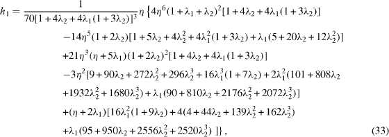
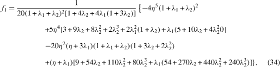
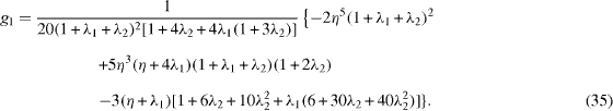
The normalized lift K and drags -f'(1), -g'(1) are then obtained from equations (24). If R = 0, we find that

$$\begin{equation} K = \infty ,\,\,\,\,\, - f'(1) = - g'(1) = \frac{1}{{1 + \lambda _1 + \lambda _2 }}. \end{equation} \tag{ 36 }$$

For large Reynolds numbers, set 1/R = ε² ≪ 1 and the governing equations become singular. We shall use the method of matched asymptotic expansions. Assume that the slip factors are of the order of unity. From equation (9) a direct expansion $h = H(\eta ) +\cdots$ gives

$$\begin{equation} HH'\,'' - H'H'' = 0. \end{equation} \tag{ 37 }$$

Relaxing the tangential velocity, the boundary conditions (14) and (15) yield

$$\begin{equation} H(0) = 0,\quad H(1) = 1,\quad H'(1) = - \lambda _2 H''(1). \end{equation} \tag{ 38 }$$

The outer solution is

$$\begin{equation} H = \frac{{\sin (c\eta )}}{{\sin c}}, \end{equation} \tag{ 39 }$$

where c is the first root of

$$\begin{equation} \tan c = \frac{1}{{\lambda _2 c}}. \end{equation} \tag{ 40 }$$

Table 1 shows some typical values.

The boundary layer is of the order of ε , and is stretched as follows:

$$\begin{equation} \eta = \varepsilon \varsigma ,\quad h = \varepsilon \phi (\varsigma ) + \cdots . \end{equation} \tag{ 41 }$$

Equations (9) and (14) give

$$\begin{equation} \phi '\phi '' - \phi \phi '\,'' = \phi ''\,'',\quad \phi (0) = 0,\quad \phi ''(0) = 0. \end{equation} \tag{ 42 }$$

The matching condition with the outer flow is

$$\begin{equation} \phi '(\infty ) = H'(0) = \frac{c}{{\sin c}}. \end{equation} \tag{ 43 }$$

The solution is

$$\begin{equation} \phi = \frac{{c\varsigma }}{{\sin c}}. \end{equation} \tag{ 44 }$$

The normalized lift is

$$\begin{equation} K = \left( {\frac{c}{{\sin c}}} \right)^2 . \end{equation} \tag{ 45 }$$

On the other hand, the outer equation for f function is

$$\begin{equation} H'F - HF' = 0 \end{equation} \tag{ 46 }$$

with the boundary condition

$$\begin{equation} F(1) = - \lambda _2 F'(1). \end{equation} \tag{ 47 }$$

We conclude that F is identically zero. The boundary condition for the boundary layer shows that the inner solution is also zero. Similarly, the function g is zero too.

For general Reynolds numbers, equations (9)–(11) and (14)–(17) are integrated numerically by the Runge–Kutta shooting method. Table 2 shows the results. These numerical results are tabulated in order to compare more precisely with approximate formulae and also with the results of future investigations.

Figure 1(b) shows a levitated circular slider of radius l which we assume is much larger than the gap width d. Align our axes on the slider such that the ground is traveling with velocity U in the x-direction. Using the similarity transform

$$\begin{equation} u = \frac{W}{d}xh'(\eta ) + Uf(\eta ), \end{equation} \tag{ 48 }$$

$$\begin{equation} \upsilon = \frac{W}{d}yh'(\eta ), \end{equation} \tag{ 49 }$$

$$\begin{equation} w = - 2Wh(\eta ). \end{equation} \tag{ 50 }$$

The Navier–Stokes equations (2)–(5) become

$$\begin{equation} - 2hh'\,'' = \frac{1}{R}h''\,'', \end{equation} \tag{ 51 }$$

$$\begin{equation} h'f - 2hf' = \frac{1}{R}f'', \end{equation} \tag{ 52 }$$

$$\begin{equation} - \frac{p}{\rho } = K\frac{{W^2 (x^2 + y^2 )}}{{2d}} + \frac{1}{2}w^2 - \nu w_z + C, \end{equation} \tag{ 53 }$$

where

$$\begin{equation} K = [h'(0)]^2 - \frac{1}{R}h'\,''(0). \end{equation} \tag{ 54 }$$

The boundary conditions are

$$\begin{equation} h'(0) = \lambda _1 h''(0),\quad h(0) = 0, \end{equation} \tag{ 55 }$$

$$\begin{equation} h'(1) = - \lambda _2 h''(1),\quad h(1) = 1/2, \end{equation} \tag{ 56 }$$

$$\begin{equation} f(0) - 1 = \lambda _1 f'(0),\quad f(1) = - \lambda _2 f'(1). \end{equation} \noindent \tag{ 57 }$$

Integrating over the bottom of the slider, the lift normalized by π ρ W² l⁴ /(4d) is K and the drag normalized by π μ Ul² /d is -f'(1).

An expansion for small Reynolds number yields the successive equations

$$\begin{equation} \fl h_0{''\,''} = 0,\quad h_0 (0) = 0,\quad h_0' (0) = \lambda _1 h_0 '' (0),\quad h_0 (1) = 1/2,\quad h_0' (1) = - \lambda _2 h_0 '' (1), \end{equation} \tag{ 58 }$$

$$\begin{equation} f_0 '' = 0,\quad f_0 (0) - 1 = \lambda _1 f_0' (0),\quad f_0 (1) = - \lambda _2 f_0' (1), \end{equation} \tag{ 59 }$$

$$\begin{equation} \fl h_1 ''\,'' = - 2h_0 h_0'\,'' ,h_1 (0) = 0,\quad h_1' (0) = \lambda _1 h_1 '' (0),\quad h_1 (1) = 0,\quad h_1' (1) = - \lambda _2 h_1 '' (1), \end{equation} \tag{ 60 }$$

$$\begin{equation} f_1 '' = f_0 h_0' - 2h_0 f_0' ,\quad f_1 (0) = \lambda _1 f_1' (0),\quad f_1 (1) = - \lambda _2 f_1' (1). \end{equation} \tag{ 61 }$$

The solutions are

$$\begin{equation} h_0 = \frac{{\eta [ - 2(1 + \lambda _1 + \lambda _2 )\eta ^2 + 3(1 + 2\lambda _2 )(\eta + 2\lambda _1 )]}}{{2[1 + 4(\lambda _1 + \lambda _2 ) + 12\lambda _1 \lambda _2 ]}}, \end{equation} \tag{ 62 }$$

$$\begin{equation} f_0 = \frac{{ - \eta + 1 + \lambda _2 }}{{1 + \lambda _1 + \lambda _2 }}, \end{equation} \noindent \tag{ 63 }$$

$$\begin{eqnarray} &&\fl h_1 = \frac{1}{{140[1 + 4\lambda _2 + 4\lambda _1 (1 + 3\lambda _2 )]^3 }}\eta \left\{ { - 2\eta ^6 (1 + \lambda _1 + \lambda _2 )^2 [1 + 4\lambda _2 + 4\lambda _1 (1 + 3\lambda _2 )]} \right.\nonumber\\ &&+ 7\eta ^4 (\eta + 6\lambda _1 )(1 + 2\lambda _2 )[1 + 5\lambda _2 + 4\lambda _2^2 + 4\lambda _1^2 (1 + 3\lambda _2 ) + \lambda _1 (5 + 20\lambda _2 + 12\lambda _2^2 )]\nonumber\\ &&- 6\eta ^2 [3 + 30\lambda _2 + 79\lambda _2^2 + 52\lambda _2^3 + 4\lambda _1^3 (13 + 91\lambda _2 + 140\lambda _2^3 ) + \lambda _1^2 (79 + 632\lambda _2\nonumber\\ &&+ 1288\lambda _2^2 + 560\lambda _2^3 ) + \lambda _1 (30 + 270\lambda _2 + 632\lambda _2^2 + 364\lambda _2^3 )]\nonumber\\ &&+ (\eta + 2\lambda _1 )[13 + 143\lambda _2 + 394\lambda _2^2 + 264\lambda _2^3 + \lambda _1 (89 + 890\lambda _2 + 2124\lambda _2^2 + 1176\lambda _2^3 )\nonumber\\ &&+ 4\lambda _1^2 (19 + 171\lambda _2 + 294\lambda _2^2 )]\}, \end{eqnarray} \tag{ 64 }$$

$$\begin{eqnarray} &&\fl f_1 = \frac{1}{{20(1 + \lambda _1 + \lambda _2 )^2 [1 + 4\lambda _2 + 4\lambda _1 (1 + 3\lambda _2 )]}}\left\{ {\eta ^5 (1 + \lambda _1 + \lambda _2 )^2 } \right.\nonumber\\ &&- 5\eta ^3 [\eta (1 + \lambda _2 ) - 2(1 + 2\lambda _2 )](1 + \lambda _1 + \lambda _2 )^2\nonumber\\ &&+ 30\eta ^2 \lambda _1 (1 + \lambda _1 + \lambda _2 )(1 + 3\lambda _2 + 2\lambda _2^2 )\nonumber\\ &&- 2(\eta + \lambda _1 )[3 + 18\lambda _2 + 35\lambda _2^2 + 20\lambda _2^3 + 2\lambda _1 (9 + 45\lambda _2 + 70\lambda _2^2 + 30\lambda _2^3 )\left. ] \right\}. \end{eqnarray} \tag{ 65 }$$

The normalized lift K and the normalized drag -f'(1) are then obtained. For R = 0, equation (36) still holds.

For large Reynolds numbers a similar outer expansion gives

$$\begin{equation} H'\,''(\eta ) = 0,\quad H(0) = 0,\quad H(1) = 1/2,\quad H'(1) = - \lambda _2 H''(1). \end{equation} \tag{ 66 }$$

The solution is

$$\begin{equation} H = \frac{{2(1 + \lambda _2 )\eta - \eta ^2 }}{{2(1 + 2\lambda _2 )}}. \end{equation} \tag{ 67 }$$

For the boundary layer, we use equation (41) to obtain

$$\begin{equation} - 2\phi \phi '\,'' = \phi ''\,'',\quad \phi (0) = 0,\quad \phi ''(0) = 0. \end{equation} \tag{ 68 }$$

The matching condition with the outer flow is

$$\begin{equation} \phi '(\infty ) = H'(0) = \frac{{1 + \lambda _2 }}{{1 + 2\lambda _2 }}. \end{equation} \tag{ 69 }$$

Thus

$$\begin{equation} \phi = \frac{{1 + \lambda _2 }}{{1 + 2\lambda _2 }}\varsigma \end{equation} \tag{ 70 }$$

and

$$\begin{equation} K = \left( {\frac{{1 + \lambda _2 }}{{1 + 2\lambda _2 }}} \right)^2 . \end{equation} \tag{ 71 }$$

Again the asymptotic solution for f is found to be zero.

For general Reynolds numbers, equations (51), (52) and (55)–(57) are integrated numerically. Table 3 shows the results.

From tables 2 and 3, the effect of slip on the dynamics properties of a slider can be summarized as follows. As the slip and/or Reynolds number increase, the normalized lift and drag decrease. The effect of slip could be significant, reducing the drag much more than the lift. The lift (per area) of a circular slider is less than that of a strip slider, while the drag remains approximately the same. The effect of Reynolds number on typical velocity profiles is shown in figure 2 for the strip slider. For low Reynolds numbers, the velocity is almost parabolic or linear. For large Reynolds numbers, a boundary layer exists near the ground. The effect of slip is shown in figure 3, where we see that the velocity distributions are very much changed. Figures 3(b) and (c) show that slip on the ground decreases the lateral velocity much more than slip on the slider. The flow is completely three dimensional. Figures 4–6 show typical pathlines in the symmetry planes y = 0 and x = 0 for the strip slider. In these figures U/W = V/W = 1. Figure 5 shows that the effect of large Reynolds numbers is to limit viscous effects to a boundary layer near the ground. Figure 6 shows that for large slip the stagnation flow is almost potential. Similar figures were obtained for the circular slider but are not presented here.

Zoom In Zoom Out Reset image size

Zoom In Zoom Out Reset image size

Zoom In Zoom Out Reset image size

Zoom In Zoom Out Reset image size

Zoom In Zoom Out Reset image size

Normally, the slip factor λ is very small, but could be large in certain instances. For example, for water injection in a gap width of 5 cm on an air lubricated film of 1 mm thickness, the slip factor is about 2.2. The slip factor can also be considered as the ratio of slip length (depth into the ground of an extrapolated velocity profile) to the gap width. For super-hydrophobic applications (Choi et al 2006) the slip length may be 20–50 μm. Thus, for micron-sized gap width, the slip factor may be of the order of 10.

The uniqueness of the Navier–Stokes equations is difficult to prove. Physically, if vorticity is being transported out of the domain, the solution is unique. This is indeed the case for slider problems.