In the following section we present four different applications of the
eatATA package to test assembly problems. The use cases were chosen to cover a broad range of contexts for ATA application: (1) A pilot study setting in which we assemble multiple test forms while depleting the item pool (without prior item calibration), (2) a typical large-scale assessment situation, in which calibrated items are assembled to blocks for a multiple matrix booklet design, (3) the assembly of multiple parallel test forms for a high-stakes assessments from a calibrated item pool, and (4) the assembly of modules from a calibrated item pool for a multi-stage assessment. To illustrate the accessibility of
eatATA compared to plain solver API’s use case (3) and (4) correspond to two of the problems used in the tutorial paper by Diao and van der Linden [
9]. Because the solver calls and the solution processing do not differ much between the minimal example and the different use cases, we primarily focus on how the constraint and objective function definitions have to be altered from application to application. Complete syntaxes for all uses cases can be found in the corresponding
Supplementary Files. 3.1. Pilot Study
Usually, when conducting a pilot study, little is known about the empirical characteristics of the item pool. Instead, the goal of a pilot study is to gather such information (e.g., response times, and missing rates) and calibrate the items. Hence, the test specifications for pilot studies often deviate substantially from test assembly specifications for operational tests. For this use case we use a simulated item pool
items_pilot, which is included in the
eatATA package. The item pool consists of 100 items with various characteristics, for example the expected response times in seconds (
“time”), the item format (
“format”), and a rough estimate of the item difficulty (
“diffCategory”), grouped into five categories. The first five items of the item pool can be seen in
Appendix B Table A1. From this item pool, we want to assemble test forms that meet the following requirements: (1) each item should appear in exactly one test form (this implies no item overlap between test forms), (2) all items should be used (
item pool depletion), (3) the expected test form response times should be as close to 10 minutes as possible, (4) the number of test forms should be determined accordingly, (5) item difficulty categories and items formats should be distributed as evenly as possible across test forms, (6) each content domain should be at least once in each test form, and (7) item exclusions should be incorporated.
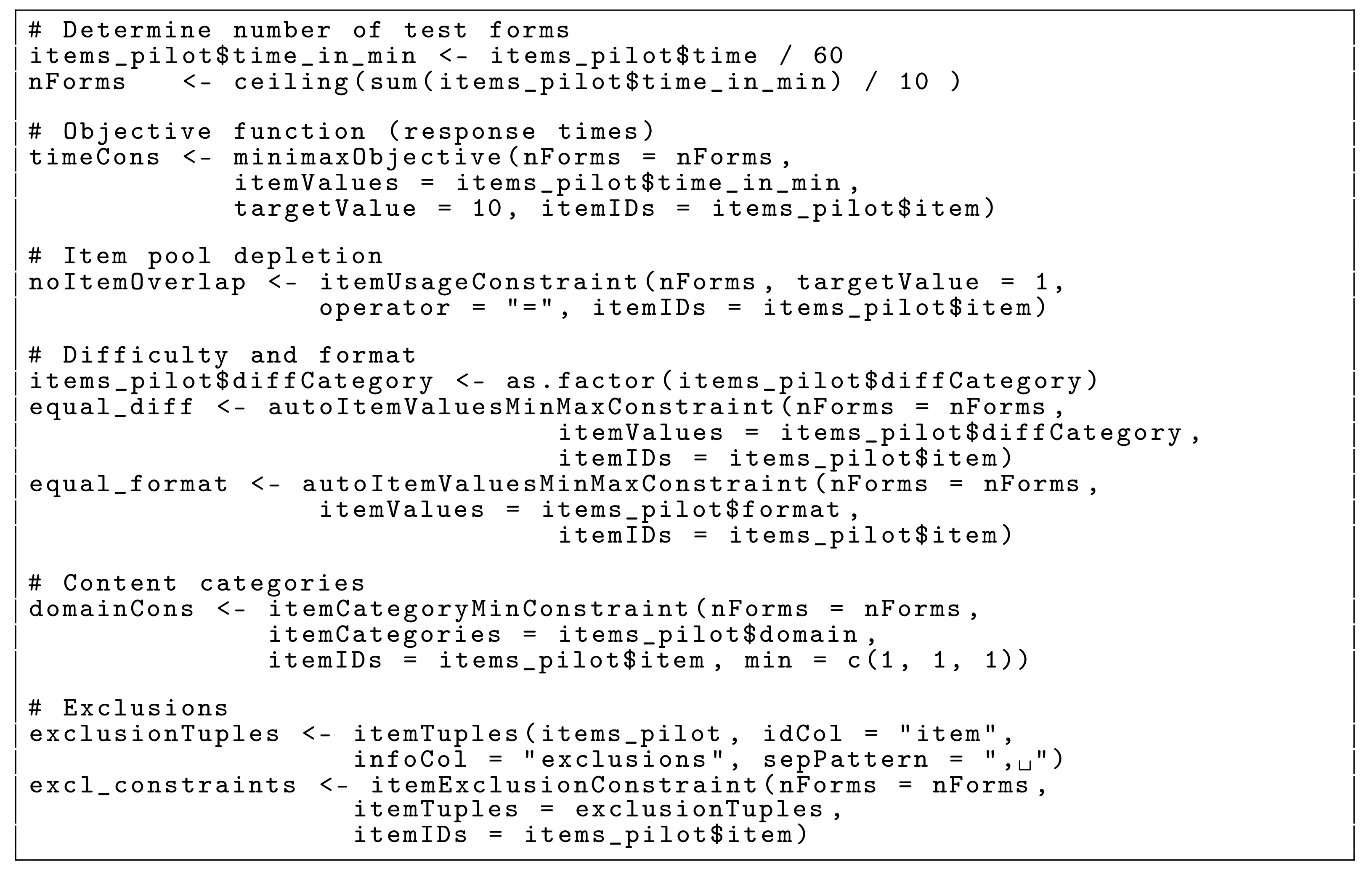
The definition of the objective function and all constraints can be seen in
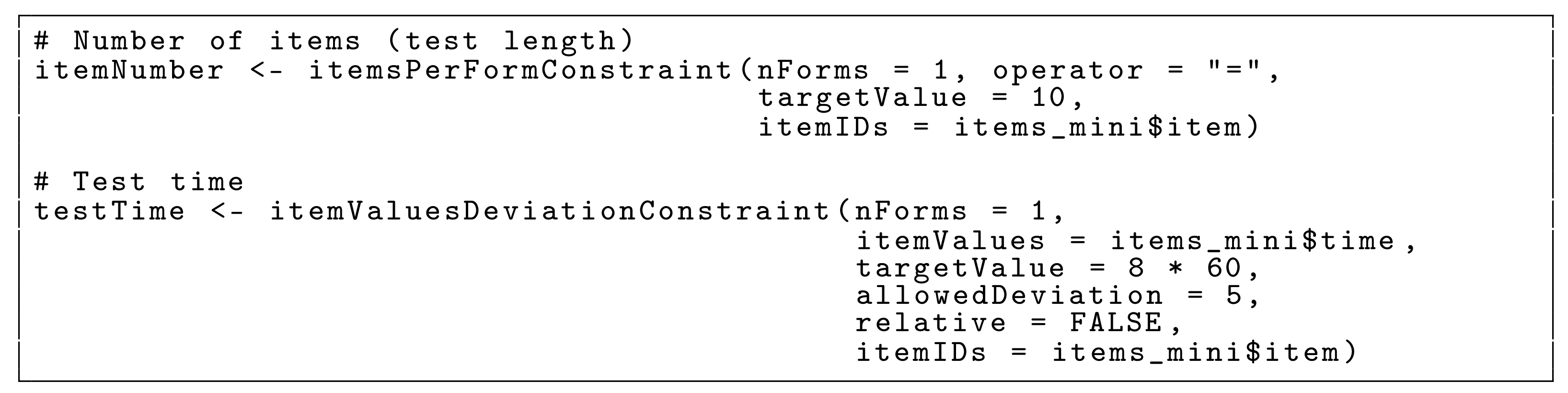
Figure 6. Among the test specifications listed above, (3) is the specification most suitable for formulation as an objective function. This means that we want to optimize the test takers’ mean test taking time and keep it as close as possible to 10 min per test form. In order to achieve this, we first transform the expected item response times to minutes. Then we calculate the ideal number of test forms by dividing the sum of all expected item response times (which is 74 min) by ten. As we prefer test forms below our target test time to test forms above our target test time, we choose the next integer above via the
ceiling() function, resulting in eight test forms. The actual objective function is defined via the
minimaxObjective() function, which allows us to specify a
targetValue. The maximum difference of test form times from this target value is then minimized.
Second, we implement test specifications (1) and (2) (item pool should be depleted and no item overlap) as constraints using a single function call to itemUsageConstraint(). The operator argument is set to “=” which means that every item will occur exactly once across all test forms. Test specification (5) refers to the difficulty column “diffCategory” as well as to the item format column “format”. For item difficulty, we define the column “diffCategory” to be a factor variable, as we do not want the numerical mean value to be equal across test forms but the distribution of distinct difficulty levels. We use the function autoItemValuesMinMaxConstraint() to determine the required targetValues automatically, after which the function directly calls the respective constraint functions using the calculated targetValues. By default, the function returns the resulting minimum and maximum levels. For example, for item difficulty, items of difficulty category 1 will occur once or twice in each test form. Alternatively, for item formats, the “cmc” format will occur four or five times in each test form. Test specification (6) requires that each domain occurs at least once in each test form. Using the itemCategoryMinConstraint() and the min argument, we define for each of the three categories (levels) of domain (“listening”, “reading”, “writing”) the minimum occurrence frequency.
Finally, we implement test specification (7), the item exclusion constraints that are captured in the
“exclusions” column of the
items_pilot data.frame. The column contains item exclusions as a single character string for each item. The items in the data set have either no exclusions (
NA), only one exclusion (e.g.,
“76”), or multiple exclusions (e.g.,
“70, 64”). As there are items with multiple exclusions, we need to separate the string into discrete item identifiers via the function
itemTuples(), which produces pairs (
tuples) of exclusive items (also called
enemy items). Using the
sepPattern argument in the
itemTuples() function, the user must specify the pattern, which separates the item identifiers within the string. These tuples can be used to define exclusion constraints in the
itemExclusionConstraint() function. The complete code for the pilot study use case, including the solver call and the solution inspection, can be seen in
Supplement S1.
3.2. LSA Blocks for Multiple Matrix Booklet Designs
Many large-scale assessments (LSAs) test forms (typically referred to as booklets) consist of multiple item blocks (also referred to as clusters). In the test assembly process, first, item blocks are assembled from the item pool and later these item blocks are combined into test forms according to so called multiple matrix booklet designs [
23]. Examples of this approach can be found in the PISA studies [
4] or are described by Kuhn and Kiefer for the Austrian Educational Standards Assessment [
3]. The present use case illustrates the first step—assembling test items to eight item blocks that fit in multiple matrix booklet designs. The second step—combining item blocks to test forms – is currently beyond the scope of
eatATA and the reader is referred to the literature on booklet designs [
24,
25].
For this purpose we assume that a pilot study has been conducted and that all required parameter estimates from an item calibration are available. We use a simulated item pool of 209 items with typical properties, which is included in the
eatATA package (
items_lsa). The first 10 items of this item pool can be seen in
Appendix C Table A2. The assembled item blocks should conform to the following test specifications: (1) blocks should contain as many well fitting items as possible, (2) hierarchical stimulus item structures should be incorporated, (3) no item overlap, (4) a fixed set of anchor items has to be included in the block assembly (if LSAs intend to measure trends between different times of measurement, new assessment cycles partially reuse items from former studies, so-called
anchor items, to establish a common scale [
26]. Usually, anchor items are chosen beforehand based on their advantageous psychometric properties), (5) the average item block times should be around 20 min, (6) difficulty levels should be distributed evenly across item blocks, (7) all blocks should contain at least three different item formats, and (8) maximally two items per block should have an average proportion of correct responses below 8 or above 92 percent.
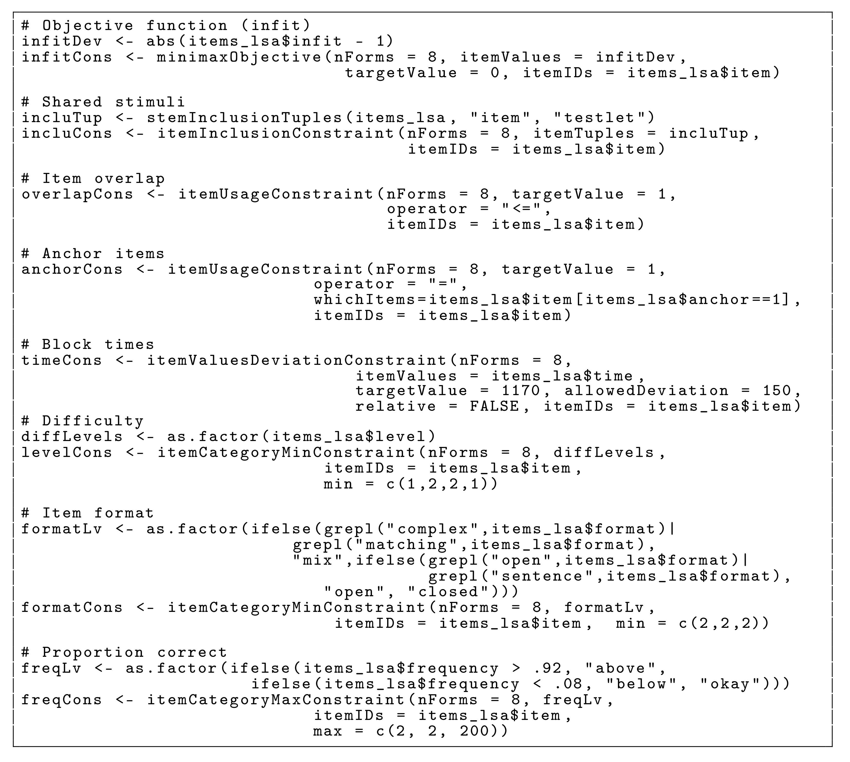
The definition of the objective function and all constraints can be seen in
Figure 7. Test specification (1) is chosen as the objective function. The infit (weighted MNSQ) is among the most widely used diagnostic Rasch fit statistics [
27] and can be found in column
“infit”. As we are only interested in absolute deviations from 1 (otherwise positive and negative deviations could cancel each other out) we create a new variable,
infitDev. The deviation of this variable from 0 is then minimized using the
minimaxObjective() function.
Test specification (2) is a common challenge for cognitive tests in LSAs, where items are usually not distinct units. Instead, multiple items share a common stimulus (e.g., a text, a picture or an auditive stimulus). Such item sets are often called
testlets. In general, testlet structures can be dealt with in different ways: (a) In the assembly, testlets can be treated as fixed structures and used as the actual units in the test assembly, (b) testlet structures can be incorporated using fixed inclusion constraints (e.g., whenever item A is chosen, items B and C that belong to the same stimulus have to be chosen, too), (c) hierarchical structures can be incorporated in the test assembly (see chapter 7 in [
1]). In the
eatATA package, options (a) and (b) are implemented and option (b) is chosen for this specific use case. Option (b) can indeed be implemented very similarly to the item exclusion constraints that were introduced in the pilot study use case. Inclusion tuples are built using the function
stemInclusionTuples() and then provided to the
itemInclusionConstraint() function.
Test specification (3) is implemented similarly as in the previous cases using the itemUsageConstraint() function. The "less than or equal" operator “<=” is used, because complete depletion of the item pool is not required. Test specification (4) refers to the forced inclusion of certain items in the block assembly, which can also be implemented using the itemUsageConstraint() function. In this specific case we specify the whichItems argument, which lets us choose to which items this constraint should apply. For this specification, the operator argument is set to “=” as the items have to appear once across the blocks.
The further test specifications are implemented in line with similar constraints in previous examples: block times, referring to test specification (5), are constrained using the itemValuesDeviationConstraint() function. Test specifications (6), (7), and (8) are implemented by transforming the respective variables to factors so we can apply the itemCategoryMinConstraint() or the itemCategoryMaxConstraint() functions. As every block should contain at least some items at the intermediate difficulty levels and also in each block at least one item at the adjacent difficulty levels, we set the min argument for this test specification to c(1, 2, 2, 1). For test specification (7), item formats are grouped into three different groups, which then are constrained by setting the minimum number of items of each group per block to two. In some LSA studies, items are flagged that have empirical proportions correct below and/or above a certain value (cf., test specification (8)). Therefore, we limit the inclusion of items that range below 8 percent and above 92 proportion correct to a maximum of two items per category per block.
The complete code for the LSA use case, including the solver call and the solution inspection, can be seen in
Supplement S2. Note that for this test assembly problem, the GLPK Simplex Optimizer finds a feasible solution very quickly but the complete integer optimization process takes a substantial amount of time, due to the large item pool, multiple assembled item blocks, and various constraints. This showcases that often setting a time limit and using a feasible but not optimal solution is sufficient in practice.
3.3. High-Stakes Assessment
This use case corresponds to Problem 1 in the paper by Diao and van der Linden [
9]. Because the item pool used in Diao and van der Linden [
9] is not freely available, an item pool was generated with similar characteristics (
items_diao in the
eatATA package). The item pool consists of 165 items following the three-parameter logistic model (3PL). Each item belongs to one of six content categories. The first five items of the generated item pool can be seen in
Appendix D Table A3. In this example, the goal is to assemble two parallel test forms with the following test specifications: (1) absolute target values for the TIFs set as
at
; minimize the distances of the TIFs of the two new forms with respect to the target at these ability values, (2) distribute the number of items per content category evenly across test forms;
Appendix E Table A4 presents the numbers of items per content category that are available in the complete item pool as well as the numbers required in each of the two forms, (3) no overlapping items, and (4) each test form should contain exactly 55 items. These specifications are directly copied from Diao and van der Linden [
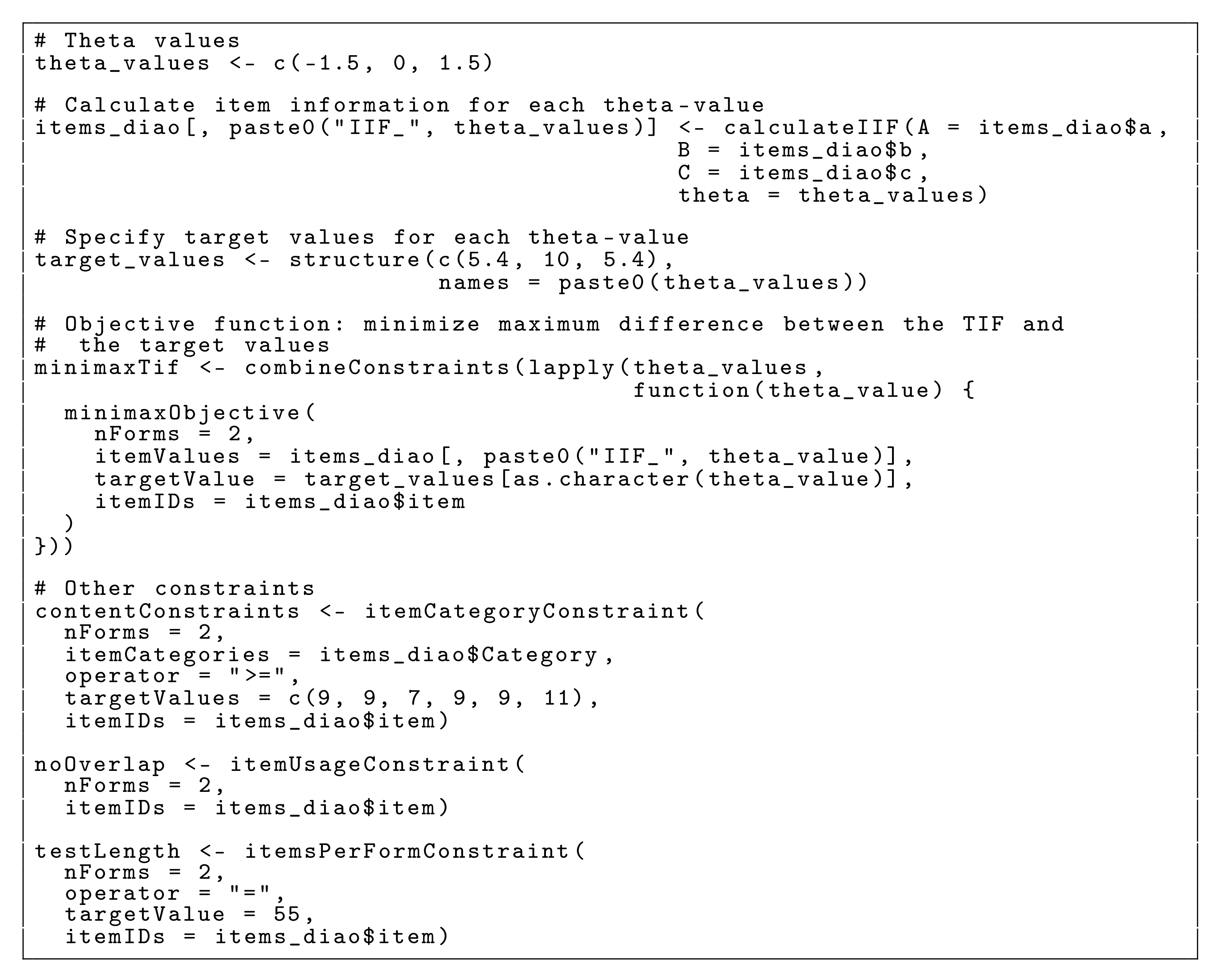
9]. The code for calculating the IIF, and setting up the minimax objective function as well as the other constraints can be seen in
Figure 8.
To implement test specification (1) we create minimax objects at each of the specified ability values, and combine them in one objective function. Hence, when solving the ATA problem, the solver will try to minimize the maximal distance between the target and the two forms at the three ability values. The implementation of the further constraints directly corresponds to formulations of test specifications in the use cases above. Therefore, further explanations on these specifications are omitted. The complete code for the high-stakes assessment use case, including the solver call and the solution inspection, can be seen in
Supplement S3.
3.4. Multi-Stage Testing
This use case covers the case of multi-stage testing and corresponds to Problem 3 in Diao and van der Linden [
9]. The use case uses the same items as use case (3), but the item pool is doubled: all items are duplicated. Hence, the item pool in this example contains 330 items following the 3PL model. Here, the goal is to assemble a two-stage multi-stage test with one routing module in the first stage and three modules in the second stage. The test specifications are: (1) the TIF of the first-stage module is required to be relatively uniform between
and
, (2) the TIFs of the second-stage modules are required to be single-peaked at
,
and
, respectively, (3) the number of item per content category should be evenly distributed across the test forms according to
Appendix E Table A4, (4) no item overlap, (5) for the first-stage module the test length should be 30 items, and (6) for each of the second-stage modules the test length should be 20 items.
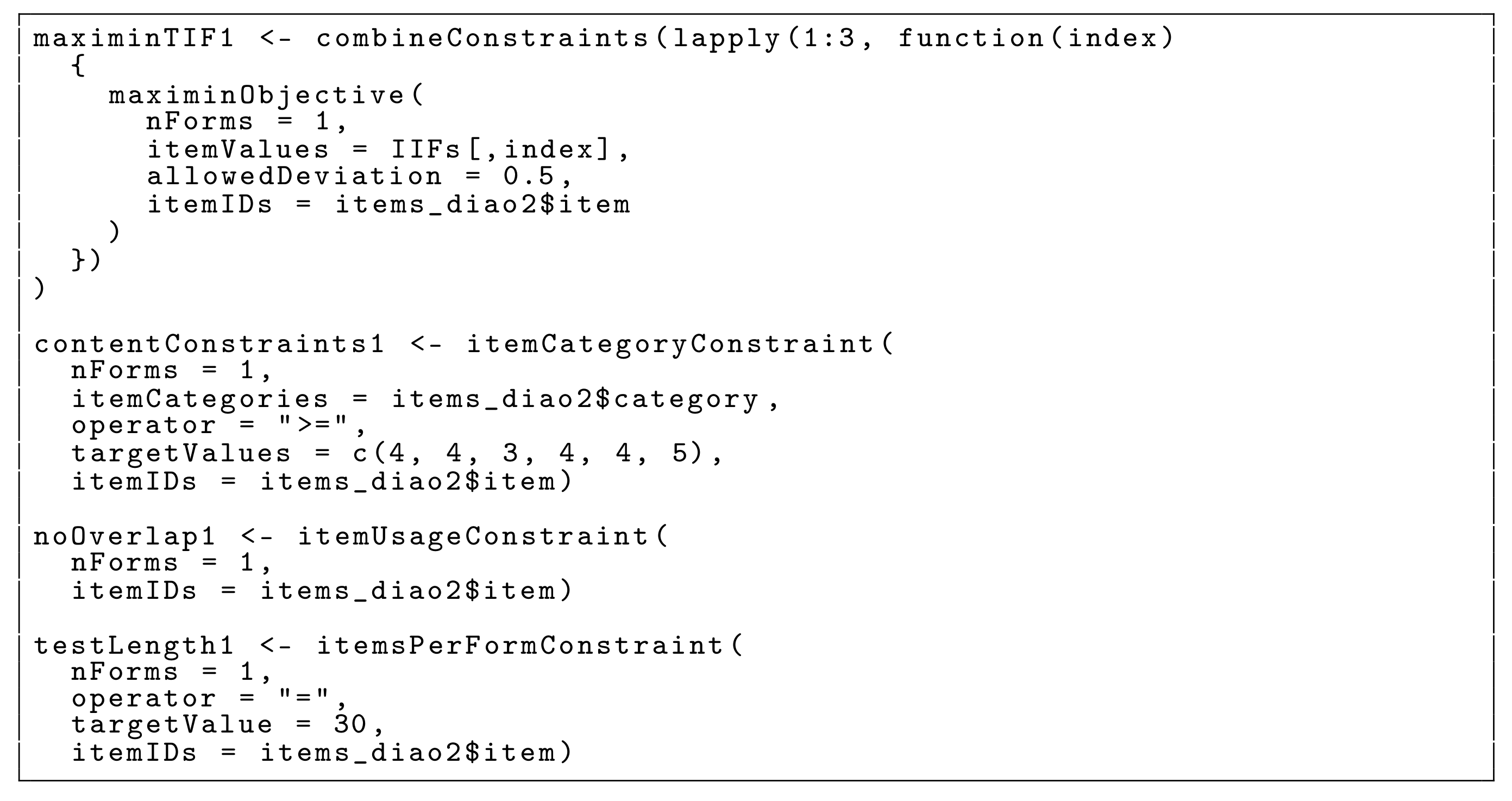
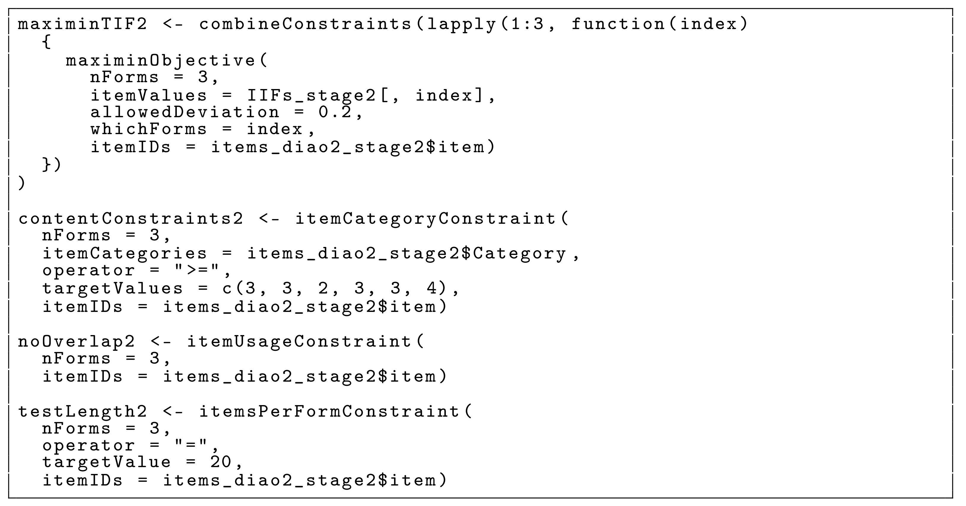
3.4.1. Original Approach
Diao and van der Linden [
9] split this assembly problem in two separate problems. In a first step, the routing module for the first stage is assembled. Thereafter, the three modules for the second stage are assembled using only the remaining items in the pool. In order to assemble the routing module with a uniform relative target, a maximin approach is used—that is, the minimum value of the TIF at the three ability values is maximized. At the same time, the TIF values at the three ability values are required to be close to each other, in order to create a TIF with a relatively flat plateau. More specifically, the TIF at the three ability values is required to be within a distance of 0.5 of each other. Hence, the
allowedDeviation is set to 0.5. The syntax for the implementation of the objective function and the constraints can be found in
Appendix F Figure A1 and
Figure A2.
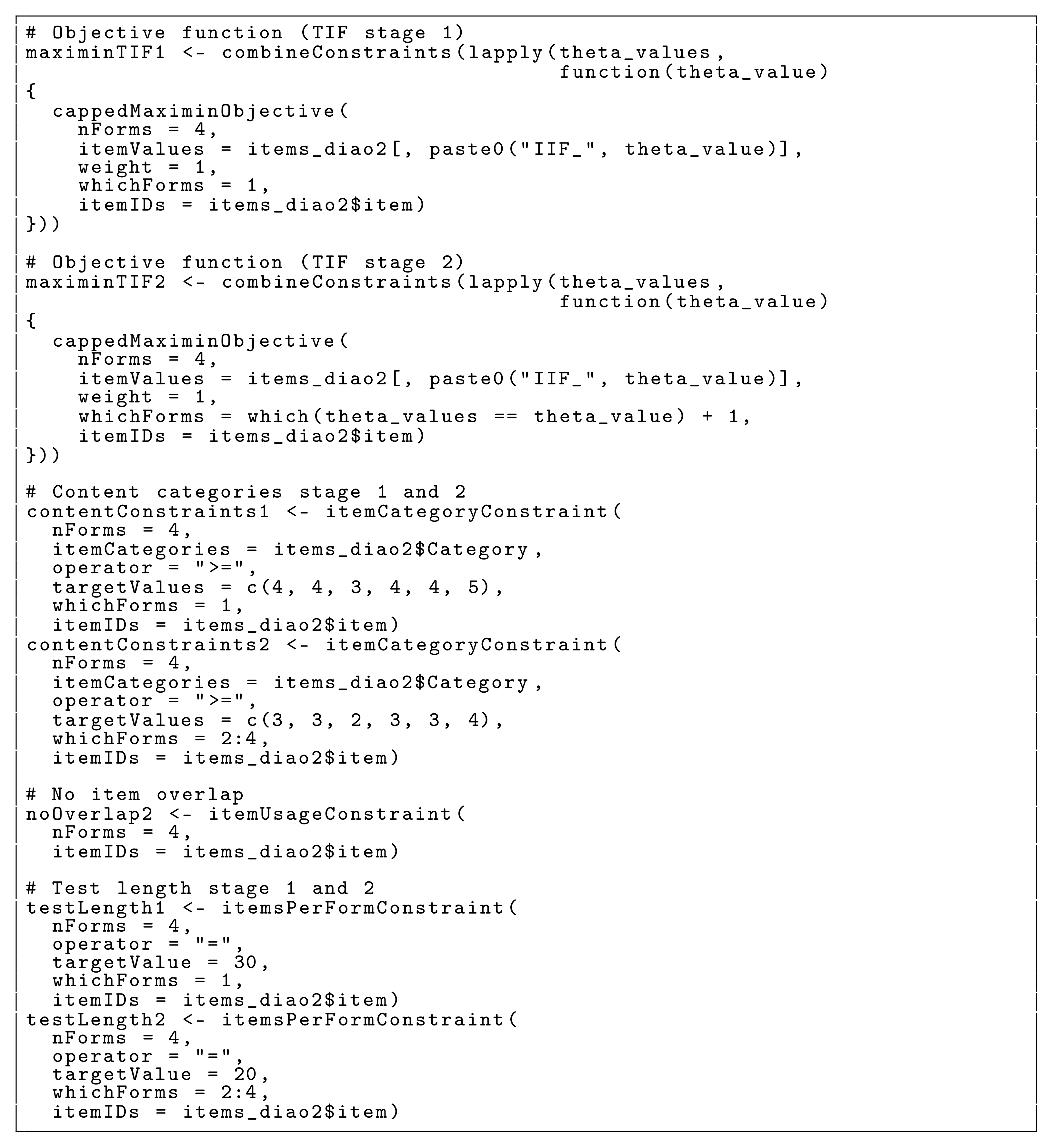
3.4.2. Combined Capped Approach
Using the eatATA package, it is possible to assemble the modules for the two stages in one combined assembly. Especially in situations with multiple stages, a simultaneous assembly may prevent infeasibility at later stages—that is, when the modules for the stages are assembled sequentially, the assembly of the first stages may deplete the item pool so that it becomes impossible to meet certain test specifications at later stages. In addition, from a practitioners perspective, a simultaneous assembly may also be easier, as the item pool does not need to be adjusted after every assembly step.
The
R syntax for the combined capped approach can be seen in
Figure 9. To implement test specification (1) we specify the maximization of the minimum TIF values at the ability values for the routing module in the first stage. Note that we do not use the original maximin approach but rather the capped maximin approach [
20]. The capped maximin approach does not require to set a maximally allowed deviation, it combines maximizing the minimal TIF with minimizing the maximal difference between the TIFs. For the modules at the second stage (test specification (2)) the capped maximin approach is also used. To combine these constraints, knowing that the obtained TIF values in the first stage and the obtained TIF values at the second stage do not need to be in the same range, we can set a weight for the TIF values. In this case, the minimal TIF in both stages can be considered equally important. Hence, the weights are set to 1 (which is the default). Because the other test specifications in
Figure 9 correspond to test specifications illustrated earlier, further explanations are omitted. The complete code for the multi-stage assessment use case, both for the original two-stage as well as the new combined assembly, with the solver call and the solution inspection, can be found in
Supplement S4.


