the Creative Commons Attribution 4.0 License.
the Creative Commons Attribution 4.0 License.
 | 30 Jul 2024
Extent of gross underestimation of precipitation in India
James Famiglietti
The underestimation of precipitation (UoP) in the hilly and mountainous parts of South Asia is estimated by some studies to be as large as the observed precipitation (P). However, UoP has been analyzed to only a limited extent across India. To help bridge this gap, watershed-scale UoP was analyzed using various P datasets within a water imbalance analysis. Among these P datasets, the often-used Indian Meteorological Department (IMD) dataset is of primary interest. The gross UoP was identified by analyzing the extent of the imbalance in the annual water budget of watersheds corresponding to 242 river gauging stations for which quality-controlled data on catchment boundaries and streamflow are available. The water year (WY)-based volume of observed annual P was compared against the observed annual streamflow (R) and the satellite-based actual evapotranspiration (ET).
Across many watersheds of both Northern and Peninsular India, spurious water imbalance scenarios (P≤R oder ) were realized. It is shown that the management of water, such as groundwater extraction, reservoir storage and water diversion, is generally minimal compared to the annual P in such watersheds. It is also shown that annual changes in terrestrial water storage are minimal compared to the annual P in such watersheds. Assuming that data on R (and, to a lesser extent, ET) are reliable, it is concluded that UoP is very likely the cause of this imbalance. Inter-watershed groundwater flow (IGF) is assumed to be negligible. While the effect of IGF on R is unknown, examples are provided which show that IGF is unlikely to be the cause of the observed imbalance in certain watersheds.
All 12 of the P datasets analyzed here suffer from UoP, but the extent of the UoP varies by dataset and region. The reanalysis-based datasets ERA5-Land and IMDAA are less affected by UoP than the IMD dataset. Based on the 30-year period of WY 1985–2014, P for the whole of India could be as much as 19 % (ERA5-Land) to 37 % (IMDAA) higher than that from the IMD, with substantial variability within years and river basins. The actual magnitude of UoP is speculated to be even greater. Moreover, trends seen in the IMD's P are not always present in ERA5-Land and IMDAA. Studies using IMD should exercise caution since UoP could lead to the misrepresentation of water budgets and long-term trends. Limitations of this study are discussed.
- Article
(3808 KB) - Full-text XML
-
Supplement
(14933 KB) - BibTeX
- EndNote


Precipitation (P) is a key component of the hydrological cycle, and changes in spatial and temporal patterns of precipitation due to climatic change is a very important area of concern (Krishnan et al., 2020). Such changes are particularly relevant for India, where a substantial portion of its population relies on an agrarian economy, which, in turn, is strongly tied to specific seasonal patterns of precipitation (Chauhan et al., 2014). Thus, the accurate measurement of precipitation and the subsequent dissemination of such measurements is important for socioeconomic purposes. Raw data from rain gauges are often compiled by government or research agencies to create precipitation products for subsequent use in hydrological and other environmental studies. Other precipitation products based on satellites, reanalysis, weather simulators, or a combination of the above sources are also available (Sun et al., 2018). Several studies have analyzed such products across the whole of India (e.g., Rana et al., 2015; Prakash, 2019; Gupta et al., 2020; Shahi, 2022) and specific regions of India (e.g., Thakur et al., 2019; Kanda et al., 2020). Within these studies, gauge-based precipitation products are often treated as reference products, or benchmarks, when evaluating satellite-based and other non-traditional datasets.
In hydrological and meteorological studies across India, the de facto benchmark dataset is the gauge-based gridded daily product from the Indian Meteorological Department (IMD) (Pai et al., 2014). However, gauge-based gridded datasets can suffer from inadequate representation of extreme events – such as those reported by King et al. (2013) in Australia; spurious trends due to changes in the locations of reporting gauges – such as those reported by Lin and Huybers (2019) using the IMD dataset; or uncertainties introduced by the relative positioning of reporting gauges – such as those reported by Prakash et al. (2019) using the IMD dataset. Moreover, measurement errors associated with gauges, such as wind-induced undercatch (Adam and Lettenmaier, 2003; Kochendorfer et al., 2017), affect the gridded products which utilize observations from such gauges. Underestimation of precipitation (UoP) has been reported in South Asia – e.g., in the upper reaches of the Ganga Basin in Nepal (Dangol et al., 2022) and in the upper reaches of the Indus Basin (Dahri et al., 2018). Studies have also explored the UoP in the mountainous regions of India using satellite and gauge-based products (Li et al., 2017). However, the UoP across the whole of India has not been thoroughly analyzed in the literature.
Goteti (2023) noted that many watersheds in the mountainous western coast of India have observed annual volumes of runoff that exceed the observed annual volume of precipitation. CWC-19 (2019) tabulated similar exceedances but did not delve into the details (e.g., Appendix R in CWC-19, 2019). It is speculated that such watersheds are affected by UoP. Some studies have developed bias-correction factors (CFs) to compensate for UoP. Such factors are often developed at the grid resolution of a reference precipitation dataset, typically with an average monthly or average annual timescale. For instance, Adam et al. (2006) and Beck et al. (2020) developed grid-based CFs utilizing the concept of the Budyko curve.
The PBCOR dataset developed by Beck et al. (2020) estimated the bias-corrected precipitation climatology corresponding to several reference climatologies (see Sect. S1 in the Supplement for further information). The ratio of the bias-corrected annual precipitation from PBCOR to that from IMD is shown in Fig. S1.2 in the Supplement. It is evident that the largest ratios occur in the wettest regions of India – the western coast of India, northernmost India and Northeastern India. If estimates from PBCOR are reasonable, they imply that the observed precipitation in these regions, and India in general, is substantially underestimated. Some of the wettest regions of India have experienced catastrophic flooding in the recent past (e.g., Hunt and Menon, 2020; Mahto et al., 2023). Thus, unbiased estimates of precipitation are important for the management of floods and other water resources. Moreover, significant decreasing trends in precipitation across India have been reported, including in the wettest parts of India (e.g., Krishnan et al., 2020). It is important to understand to what extent such trends are affected by UoP. The identification and quantification of UoP across India is important for many reasons but has not received much attention from the scientific community. Filling this void is the motivation behind this study.
The following conventions are used throughout this paper. The words “catchment” and “watershed” are used interchangeably for smaller watersheds, while the word “basin” is reserved for larger watersheds – e.g., the Indus Basin. A reference time period often used when analyzing hydrological variables is the water year (WY). A WY is defined here as the period starting from 1 June and ending on 31 May of the following year. For example, WY 2020 spans the period from 1 June 2020 to 31 May 2021. This definition is consistent with the definition of WY often used by Indian agencies (e.g., CWC-19, 2019).
2.1 Study domain, river gauging stations and catchment boundaries
The study domain includes the river basins that span India, including the catchment areas that fall outside of the political boundaries of India (Fig. 1). The boundaries of the river basins used here are generally consistent with those used by India's Central Water Commission (CWC). Consistent with the CWC, adjacent watersheds in some regions were pooled to create composite river basins, such as west-flowing rivers (WFR) north and south, east-flowing rivers (EFR) north and south, and west-flowing rivers of Kutch (WFR Kutch). The catchment boundaries used here are from the GHI dataset (Goteti, 2023), a quality-controlled dataset on India's river gauging stations, catchment boundaries and hydrometeorological time series. However, the GHI dataset is limited to Peninsular India. The catchment boundaries for the Northern Indian watersheds were derived using the HydroSHEDS suite of products, using the same procedures as the GHI dataset. Station descriptions available from the CWC were validated using online maps (e.g., Google Maps). Stations were then relocated to the closest point on the river network. The watershed draining into this relocated point and all of the upstream watersheds were recursively identified using geographic information system (GIS) software. Catchment areas for the delineated watersheds were validated against those reported by the CWC.
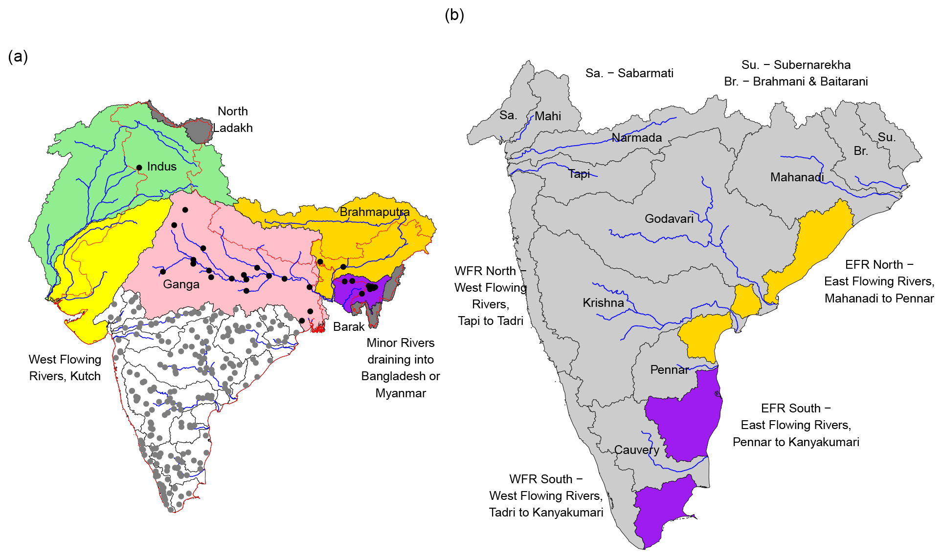
Figure 1(a) Major river basins spanning India. The shaded basins are transboundary basins. Stations with daily streamflow data (grey dots) are from the GHI dataset (Goteti, 2023), and stations with only annual streamflow data (black dots) are from CWC-19 (2019). (b) River basins of Peninsular India. Some basin names have been shortened for ease of display within the map, with the complete names shown next to the map.
The river basins of Peninsular India, the non-shaded region in Fig. 1a, have daily streamflow data that are available through India's Central Water Commission (CWC). Limited streamflow data are available for the river basins of Northern India (shaded regions in Fig. 1a). The stations used here were chosen such that the catchment area discrepancy between the GHI and CWC datasets is less than 5 %, and there was at least 5 years of observed streamflow data with minimal missing records. A total of 242 stations are used in this analysis, with 213 of these stations located in Peninsular India and 29 in Northern India (dots in Fig. 1a). The number of stations within each basin and other pertinent information are summarized in Tables S2.1 and S2.2.
2.2 Precipitation
The selected P datasets used here are outlined in Table 1 and are briefly described here. In addition to these datasets, the PBCOR dataset is used as a reference climatology in certain parts of this analysis. Additional information on the PBCOR dataset is provided in Sect. S1, while additional information on P datasets is presented in Sect. S3.
Yatagai et al. (2012)Funk et al. (2014)Xie et al. (2017)Muñoz-Sabater et al. (2021)Kubota et al. (2020)Pai et al. (2014)Rani et al. (2021)Huffman et al. (2020)Beck et al. (2019)Sadeghi et al. (2021)Brocca et al. (2019)Abatzoglou et al. (2018)Table 1The P datasets analyzed here and relevant information. The input used in the creation of each dataset is indicated by one or more of “G” (gauge), “O” (observation-based data product), “R” (reanalysis) and “S” (satellite). In the time span, the end year is left blank when a dataset extends to the present.
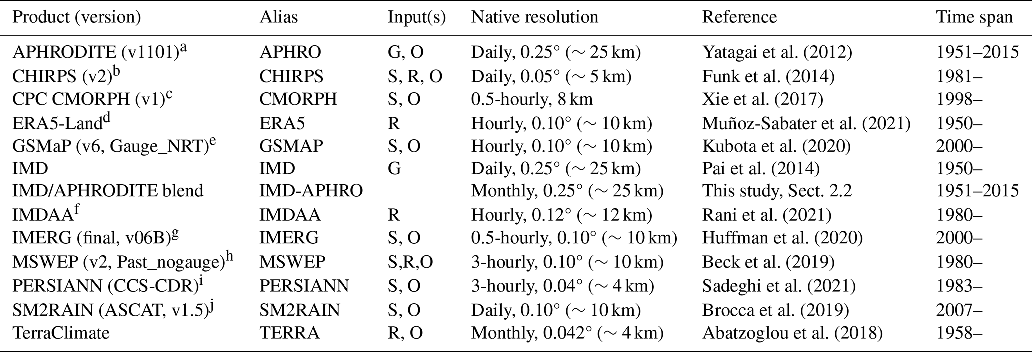
a Asian Precipitation – Highly-Resolved Observational Data Integration Towards Evaluation of Water Resources. b Climate Hazards Group InfraRed Precipitation with Station data. c Climate Prediction Center Morphing Technique. d European Centre for Medium-Range Weather Forecasts (ECMWF) land component of the fifth generation of European ReAnalysis (ERA5). e Global Satellite Mapping of Precipitation. f Indian Monsoon Data Assimilation and Analysis reanalysis. g Integrated Multi-satellitE Retrievals for Global precipitation measurement. h Multi-Source Weighted-Ensemble Precipitation. i Precipitation Estimation from Remotely Sensed Information using Artificial Neural Networks (Cloud Classification System–Climate Data Record). j Soil Moisture to Rain (Advanced Scatterometer, v1.5).
The P datasets used here were often identified in the recent literature as being reasonable representations of the observed P, and they range in spatial resolution from about 4 to 25 km and in temporal frequency from half an hour to a month. Datasets included here are based on rain gauges (e.g., the IMD dataset), reanalysis (e.g., ERA5-Land), satellites, or a combination of sources (e.g., CHIRPS). The IMD gauge-based dataset is of primary interest here, since it is an often-used benchmark that is employed in a number of studies.
The reader should note that while the IMD dataset is limited to India's political boundaries, the rest of the P datasets are not. However, certain river basins of India extend beyond India's boundaries and are part of this analysis. To enable an appropriate comparison between datasets, the IMD dataset is complemented, where needed, with the APHRODITE dataset (Yatagai et al., 2012). The APHRODITE dataset was chosen for several reasons: it is also based on rain gauge data, similar to the IMD dataset; its spatial and temporal resolution are the same as the IMD dataset's resolution (0.25° or ∼25 km and daily); and studies in the literature have found that APHRODITE compares reasonably well with the IMD dataset across many parts of India (e.g., Prakash et al., 2015b). While limitations with APHRODITE are discussed by such studies, it is assumed to be the best gauge-based alternative to the IMD dataset.
For those regions where data from the IMD are unavailable, grids from APHRODITE were identified, and then the data from those grids was interpolated to align with the IMD dataset grid. Finally, a blended product called IMD-APHRO which spanned the entire study domain was created. In the remainder of this paper, unless otherwise stated, IMD-APHRO refers to the blended product created here, and IMD refers to the product confined to India's political boundaries. Also, in the remainder of this paper, each P product is referred to by its alias (see Table 1).
2.3 Evapotranspiration
Two datasets were considered for this analysis, based on their usage in studies across India (Table 2) – the Numerical Terradynamic Simulation Group (NTSG) at the University of Montana (Zhang et al., 2010) and the Global Land Evaporation Amsterdam Model (GLEAM) (Martens et al., 2017; Miralles et al., 2011) datasets. GLEAM provides estimates of the different components of ET, including transpiration, bare-soil evaporation, interception loss, open-water evaporation and sublimation. A comparison of NTSG and GLEAM indicates that they are generally consistent with each other across several basins (Sect. S4). However, estimates from GLEAM tend to be lower than those from NTSG. GLEAM was the primary dataset used here because of its longer time span and its availability up to the present time.
Zhang et al. (2010)Martens et al. (2017)Miralles et al. (2011)Table 2The evapotranspiration datasets analyzed here and relevant information. In the time span, the end year is left blank when a dataset extends to the present.
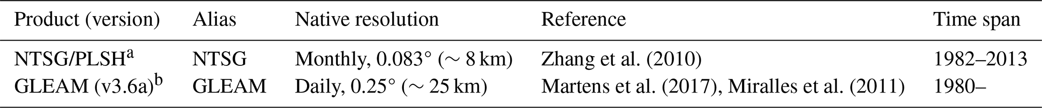
a Numerical Terradynamic Simulation Group (NTSG) Process-based Land Surface evapotranspiration/Heat (PLSH) fluxes algorithm. b Global Land Evaporation Amsterdam Model.
2.4 Other data
2.4.1 Elevation, land cover and land use
Figure 2a shows the variability in elevation across the study domain. The dominant features include the Himalayas in the northern and northeastern regions, the mountains (or ghats) along the western and eastern coasts of India, the plains of the Ganga and Brahmaputra basins, and the Deccan Plateau in Peninsular India.
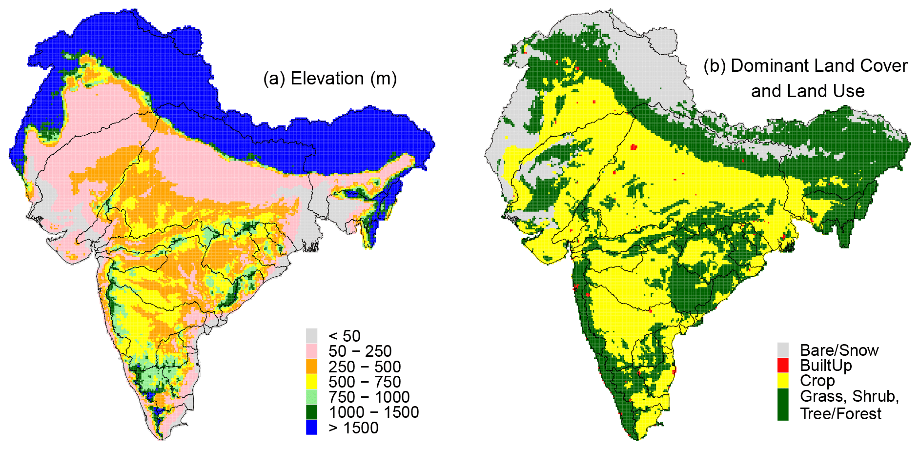
Figure 2(a) Elevation based on HydroSHEDS 500 m topographic data. For ease of display, 500 m data are aggregated to 10 km resolution and the maximum value within each 10 km grid is displayed. (b) Major land-cover and land-use types based on PROBA-V 100 m data. For ease of display, 100 m data are aggregated to 10 km resolution and the dominant value within each 10 km grid is displayed.
The high-resolution (100 m) global dataset based on the PROBA-V satellite (Buchhorn et al., 2020) was used to identify the dominant land-cover and land-use types. Figure 2b shows the dominant land-cover and land-use types. For the purpose of this analysis, the land-cover types of grass, shrubs, and trees/forest were pooled into one category.
2.4.2 Water management
The water management considered here includes groundwater extraction, diversions (imports and exports), and reservoir storage, which are summarized in Fig. 3. A detailed description of these data is provided in Sect. S5. Groundwater extraction and recharge estimates are available from India's Central Ground Water Board (CGWB) for select years. The extent of annual groundwater extraction is quantified as a fraction of the annual P. Similarly, basin-scale imports and exports from CWC-19 (2019) are expressed as a fraction of the annual P. Information on large dams and reservoirs in India was obtained from the National Registry of Large Dams (NRLD, 2019). For each of the 242 watersheds used here, the cumulative live storage capacity from all dams present within the watershed is expressed as a fraction of the annual P.
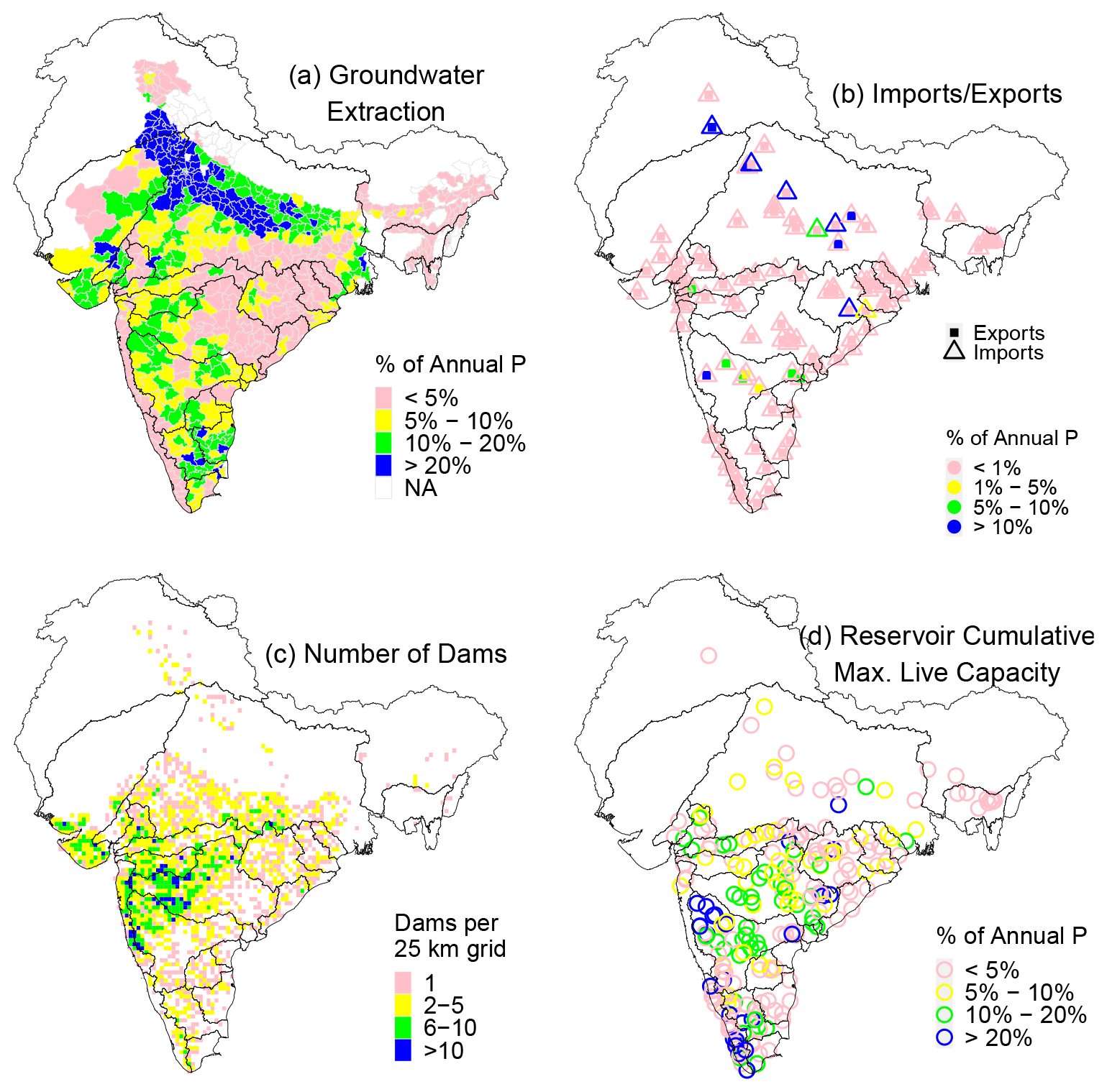
Figure 3(a) Districtwise annual groundwater extraction as a percent of the annual P; (b) basin-scale imports and exports as a fraction of the annual P; (c) density of dams and reservoirs, represented as the number of dams per 0.25° (about 25 km) grid; and (d) cumulative maximum live storage capacity of each watershed expressed as a fraction of the annual P for WY 2019.
Figure 3a shows that groundwater extraction can be a substantial fraction of the annual P in certain parts of India, but it is minimal in the mountainous and wet regions of India – the western coast of India, northernmost India and Northeastern India. Similarly, water diversions are highest in the agricultural regions of the Ganga Basin and the interior parts of Peninsular India. The highest density of dams is in arid Western India, while the lowest density occurs in the plains and mountains of Northern India. There are some watersheds in coastal Peninsular India, where reservoir storage is a significant portion of the annual P, but most of the other watersheds are minimally impacted by such storage.
2.4.3 Changes in terrestrial water storage (TWS)
Changes in terrestrial water storage (TWS), inferred from the Gravity Recovery and Climate Experiment (GRACE) satellite mission (Tapley et al., 2004), are useful for identifying regions where large-scale water management is causing substantial changes to the natural hydrologic cycle (e.g., Famiglietti, 2014; Rodell et al., 2009). TWS includes water stored below the ground, on the ground and above the ground. GRACE-based TWS anomalies from the Center for Space Research (CSR) (Save et al., 2016; Save, 2020) were used to estimate the change in annual TWS (or ΔTWS) as a fraction of the annual P (see Sect. S6). Figure 4 shows the maximum and minimum ΔTWS over the period WY 2002–2014. The magnitudes of such changes for most of the study domain are within +20 % or −20 % of the annual P. However, there are regions, such as Northwestern, Northern and Eastern India, where the magnitudes of such changes are larger than 20 % of the annual P.
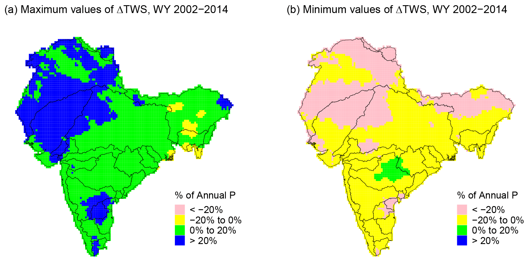
Figure 4(a) Gridwise maximum values of annual ΔTWS for WY 2002–2014. (b) Same as (a) but for the minimum values.
The overall objective is to analyze the spatial extent and magnitude of the watershed-scale or gross UoP in India and not the station-scale UoP. A station-scale analysis of UoP is beyond the scope of this study because the data needed are unavailable. The UoP is identified by analyzing the water balance (or lack of it – i.e., an imbalance) where reliable hydrometeorological data are available. By eliminating two potential causes of this annual water imbalance – namely, large-scale management and substantial changes in annual terrestrial water storage (ΔTWS) – it is concluded that the likely cause of the imbalance is UoP. Other potential causes of a water imbalance are also discussed.
The overall methodology and the specific objectives are illustrated in the flowchart in Fig. 5. The specific objectives are: (1) to analyze the annual water budgets of watersheds using IMD as the source of P and to identify the imbalanced watersheds; (2) to investigate the large-scale management and annual ΔTWS in those watersheds and to attribute the cause of the imbalance to UoP if management and ΔTWS are found to be relatively minimal; and (3) to analyze the extent of the UoP within other state-of-the-art P products and to compare it against the UoP in IMD to identify reasonable alternatives, if any, to IMD.
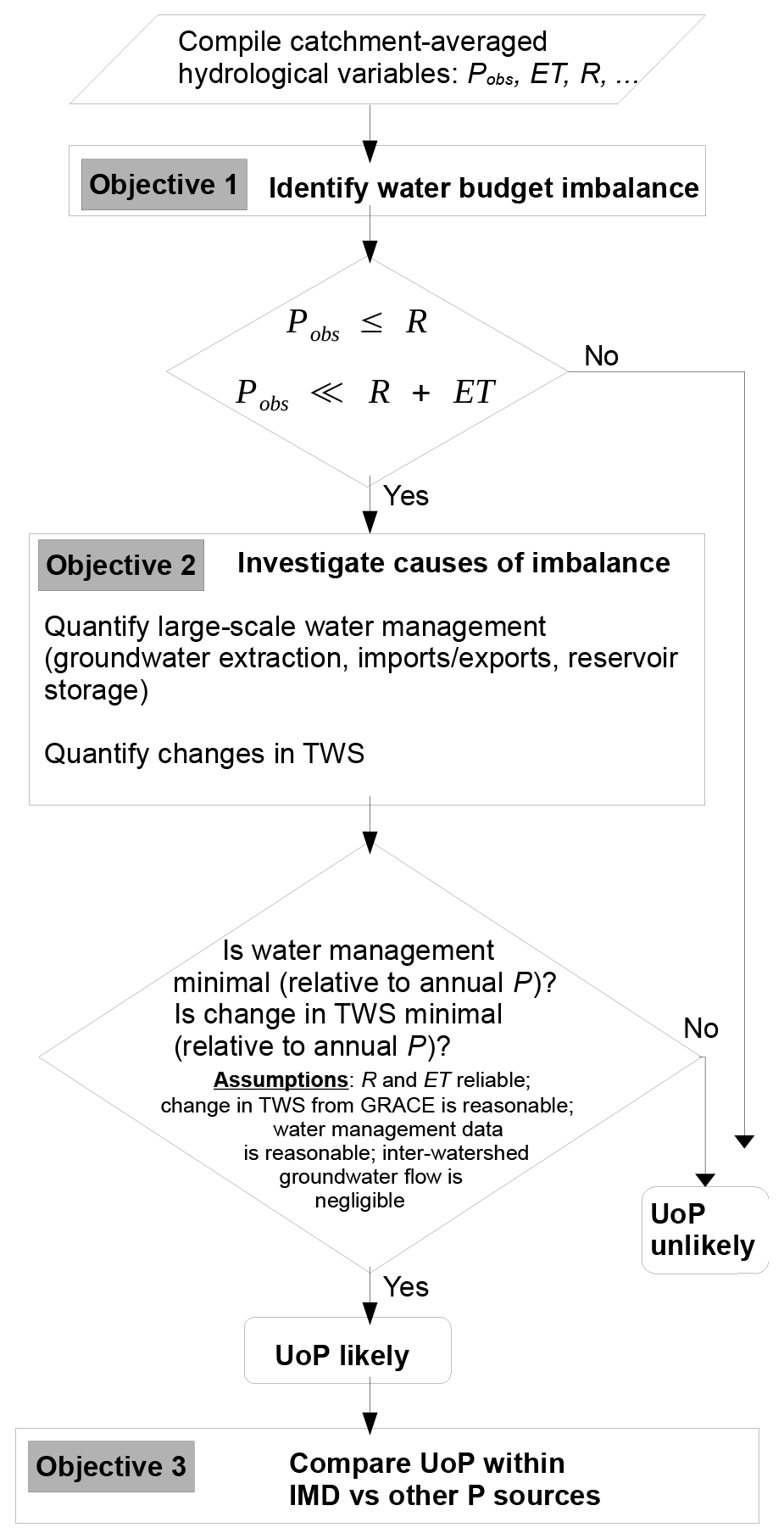
Figure 5Flowchart showing the overall objectives, the methods used to achieve those objectives and the major assumptions made in this study.
In this study, UoP is said to occur when the observed annual P (Pobs) is less than the actual annual P (Pact) averaged over the entire watershed (Pobs<Pact). Since Pact is unknown, expected empirical relationships between Pobs and other hydrological fluxes are examined to identify the gross UoP. Watersheds affected by UoP would be those where the balance between inputs (Pobs) and outputs (e.g., R and ET) cannot be reconciled despite reasonably accounting for changes in TWS or disruptions to the natural balance caused by large-scale management. Watersheds are assumed to have negligible flow across topographic boundaries – i.e., inter-watershed groundwater flow (IGF) is ignored. The particular UoP scenarios analyzed here are described in Sect. 3.1. The methodology used to compile the data needed for such an analysis is described in Sect. 3.2.
3.1 Water imbalance scenarios
In order to take advantage of the datasets on TWS anomalies and water management discussed in Sect. 2.4, the traditional annual water balance equation is formulated in two different ways in the following discussion.
Under natural circumstances, one could express the annual water balance of a watershed by assuming that the net change in terrestrial water storage (ΔTWS) is the imbalance between the total actual P (Pact), the output fluxes of R and ET, and inter-watershed groundwater flow (IGF):
TWS is the sum of all the potential water reservoirs – groundwater, soil moisture, snow water equivalent, surface water, land ice and water in the biomass (Humphrey et al., 2023). Watershed boundaries do not always coincide with underlying aquifer boundaries, and IGF could play an important role in the watershed's water balance (e.g., Fan, 2019; Liu et al., 2020). However, in the absence of field data on groundwater flow pathways, it is not possible to quantify the effect of IGF on the water balance. IGF is assumed to be negligible. The implications of this assumption are discussed in Sect. 5.1.2.
If one were to account for the effects of management, ΔTWS would represent changes due to both natural and human-related causes such as groundwater extraction, reservoir storage and diversions. Under such circumstances, after ignoring IGF, one could reformulate Eq. (1) as Eq. (2). Net surface water diversions are represented by two terms: Exports (net loss of water) and Imports (net gain of water). The terms Pact, R, ET, Exports and Imports are non-negative. ΔTWS is positive if there is a net increase in TWS and negative if there is a net decrease in TWS.
Rearranging Eq. (2) results in Eq. (3). The equality in Eq. (2) has been replaced with an approximation in Eq. (3) because the data needed, if available, are often not at the spatial or temporal resolution required to accurately balance the water budget.
There is another way, although more approximate than Eq. (3), of formulating the annual water balance. Management of water is present in many parts of India and includes groundwater extraction, reservoir storage and diversions (CWC-19, 2019). To take advantage of these data on management, the annual water balance is approximated as Eq. (4). Groundwater storage changes – both natural (ΔGW natural) and human-caused changes (ΔGW human) – are included. Changes to reservoir storage (ΔReservoir) and diversions (Exports and Imports) are also explicitly included. In Eq. (4), both ΔGW terms are positive if there is a net aquifer recharge and negative if there is a net aquifer depletion. Thus, the groundwater extraction presented in Fig. 3 would be a negative quantity. ΔReservoir is positive if there is a net increase in reservoir storage and negative if there is a net decrease in storage.
The reader should note that Eqs. (3) and (4) are separate, but useful, ways of analyzing the water budget. While ΔTWS in Eq. (3) includes changes in all potential water reservoirs, Eq. (4) is an approximation and does not adequately capture the effect of snow processes, does not include water stored as soil moisture, and does not capture all the effects of management. The reader should also note that hydrologic analyses often make the a priori assumption that the net annual change in storage (ΔTWS or ΔGW) is negligible. This study does not make such an assumption within Eqs. (3) and (4).
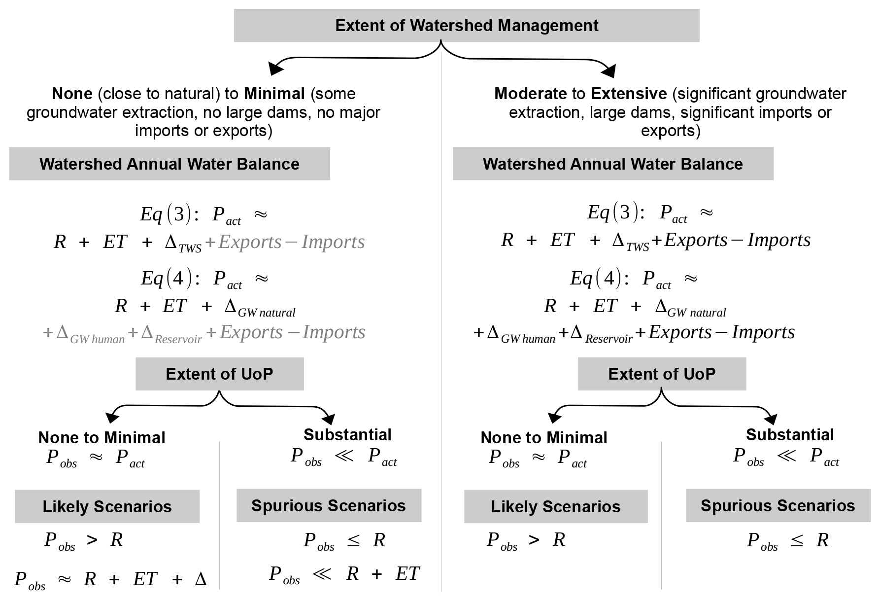
If UoP is absent (i.e., Pobs≈Pact), then, based on Eqs. (3) and (4), it is reasonable to expect R to be only a portion of Pact, regardless of the extent of management. If the effects of management – the two rightmost terms in Eq. (3) and the four rightmost terms in Eq. (4) – are relatively small compared to Pact, then it is also reasonable to expect Pact to approximately equal , where Δ is either ΔTWS oder ΔGW natural. As discussed later in this section, for most watersheds in the study domain, a reasonable upper bound on the magnitude of ΔTWS (and ΔGW natural) is 20 % of Pobs. The above expectations are illustrated by the “likely scenarios” in Fig. 6.
If UoP is present (i.e., Pobs≪Pact), one could potentially realize the “spurious scenarios” of Pobs≤R and (see Fig. 6) when the extent of management is minimal. If, on the other hand, management is moderate to extensive, it is difficult to generalize the relationship between the relative magnitudes of Pact, R and ET since R and ET are no longer constrained by the natural water balance. The spurious scenarios in this situation only include the case where Pobs≤R. The word “minimal” is used in a relative sense when the overall effect of annual management at the watershed scale relative to the annual Pobs is minimal. It should not be interpreted as the effect of local management on specific storm events.
The two specific scenarios investigated here are based on the spurious scenarios in Fig. 6. The annual Pobs is less than or equal to R in Scenario I.
Thus, the annual runoff coefficient is at least 1 in Scenario I. This scenario could be realized regardless of the extent of management outlined in Fig. 6. Such a scenario was also used by other studies (e.g., Beck et al., 2020) to identify UoP. However, instances where the annual runoff coefficient is less than 1 but still spuriously high (e.g., 0.95) are excluded by Scenario I. Scenario II attempts to include such instances.
Moreover, Scenario II is also intended to capture instances where the sum of R and ET greatly exceeds Pobs. If UoP is present, relatively high values of R combined with reasonable estimates of ET result in the sum of R and ET greatly exceeding Pobs. The formulation of Scenario I exactly follows the first of the spurious scenarios in Fig. 6. The second of the spurious scenarios in Fig. 6, , is not an exact mathematical relationship. It is made exact by the use of heuristics. The rationale behind such heuristics is presented in the following discussion.
The typical wet season runoff coefficient for the whole of India was estimated to be about 0.38 by Gupta et al. (2016). The basin-scale average annual runoff coefficient was estimated by Xiong et al. (2022) to range from 0.10 to 0.40 for several large river basins of India, with higher coefficients for the Indus and Brahmaputra basins. Considering the magnitudes of those estimated runoff coefficients, a coefficient of 0.70 was assumed to be a reasonable lower bound for identifying spuriously high annual runoff coefficients.
As shown in Fig. 4, for regions that have hilly terrain or are covered by forests, the magnitude of ΔTWS is typically within 20 % of the annual Pobs. Watershed management is represented by the four rightmost terms in Eq. (4): ΔGW net recharge, ΔReservoir, Exports and Imports. In the regions that have hilly terrain or are covered by forests (Fig. 2), where management can be assumed to be minimal, the magnitude of the individual effect of each type of management is typically less than 5 % of Pobs (Fig. 3). A reasonable upper bound on the cumulative effect of the four rightmost terms in Eq. (4) is also 20 % of the annual Pobs. Thus, when management can be considered minimal, it is reasonable to expect R+ET to have a maximum value of 1.20×Pobs. This is the justification for the heuristic of 1.20 in Scenario II. As mentioned earlier, “minimal” management is used in the context of the overall effect of annual management at a watershed scale relative to annual Pobs. For instance, a 20 % management effect of the annual Pobs in a watershed with 0.4 as the runoff coefficient translates to a 50 % () effect on the annual R. Thus, minimal management could still have a substantial effect on the annual R.
This study identifies UoP by first identifying individual years within watersheds where Scenario I or II is realized. Then, it proceeds to investigate the extent of management and extent of ΔTWS within those imbalanced watersheds. If management and ΔTWS are deemed minimal relative to annual P, then it is concluded that the likely cause of the spurious imbalance is UoP.
3.2 Time series compilation
In order to investigate the abovementioned scenarios, annual time series of all the relevant terms need to be compiled. All of the variables needed are expressed in the same units of volume. Observed daily streamflow (R), available in units of m3 s−1 was aggregated to cumulative monthly and annual volumes of million m3 s−1 (MCM per month and MCM per year, respectively). Gridded data on Pobs and ET, available in units of depth per unit area per month (e.g., mm per month), were also aggregated to watershed-scale monthly and annual volumes. The process of aggregating grid-based products to a watershed involves identifying the spatial overlap between the grids and the watershed. Such relationships were identified using a GIS analysis. Grid-specific fractional areas were used in the process of aggregation. A schematic illustrating the process of aggregation is shown in Sect. S7. The time series needed were compiled for each of the 242 watersheds analyzed here. P datasets are often available up to the current year, but the latest year for which observed R data are available is WY 2017, and ET data since WY 1980 are available. The time span of the data compiled here is WY 1980 to 2017 (38 WYs), whenever data are available.
The results presented here follow the specific objectives outlined in the Introduction. The observed UoP within the IMD-APHRO dataset is discussed in Sect. 4.1, which includes an example illustrating the spurious water imbalance potentially caused by UoP and considers the spatial extent of imbalanced watersheds. The hydroclimatological characteristics of such imbalanced watersheds, including the extent of management, are discussed in Sect. 4.2. The extent of UoP within all P datasets is compared in Sect. 4.3. Using select datasets which present less UoP than IMD-APHRO, gridwise potential correction factors (CFs) associated with IMD are estimated in Sect. 4.4. Basin-scale potential CFs are also discussed in Sect. 4.4.
4.1 Imbalanced watersheds identified using IMD-APHRO
An example of Scenario I is shown in Fig. 7 for the Bantwal station on the Nethravathi River in the WFR south basin. The annual time series is shown in Fig. 7a, while the monthly time series for select years is shown in Fig. 7b. There are several WYs where the total annual volume of P is less than the total observed R, such as WYs 2011–2013 in the recent past. The total live capacity of all upstream reservoirs is 0 since there are no dams in this watershed. The monthly time series is also shown in for select years (WYs 2011–2015; Fig. 7b). The strong seasonal pattern imposed by the summer monsoon is evident, with the months of June to September having the highest values of P and R. There are several months within each year where the observed R is greater than P. It is useful to note that the above spurious relationship in which the annual R exceeds the annual P for the Bantwal watershed was also tabulated by CWC-19 (2019) (see their Appendix R, Table R-2), based on the same P and R data sources as those used here.
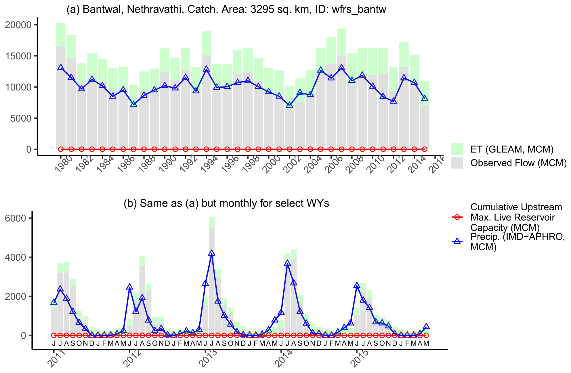
Figure 7(a) Example showing the imbalance scenario P≤R (Scenario I) for Bantwal station on the Nethravathi River in the WFR south basin. The annual R (grey bars) exceeds annual P (blue line) in certain years. ET (green bars) and cumulative reservoir storage capacity (red line) are also shown for reference. (b) Monthly volumes instead of annual volumes for select WYs. Months are indicated by initials and follow the June–May WY convention.
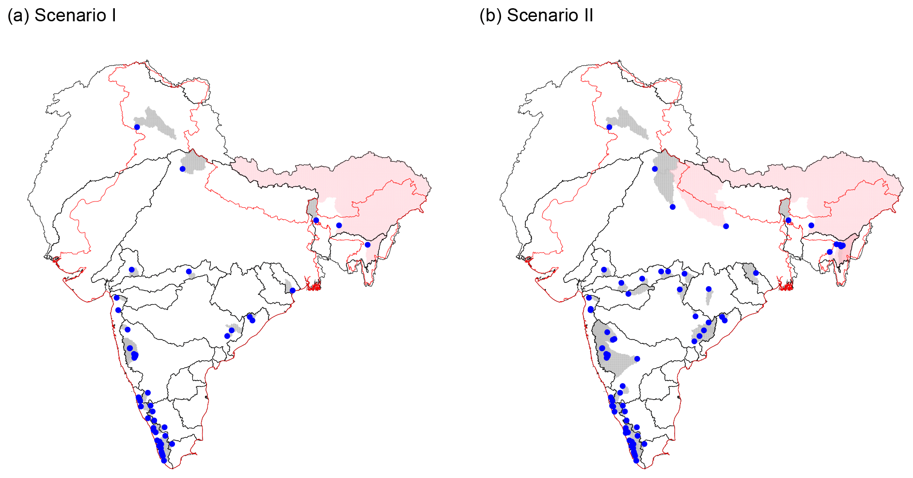
Figure 8(a) Imbalanced watersheds from Scenario I (grey-shaded regions) and the gauging stations (blue dots) at the outlets of those watersheds. Watersheds shaded in pink have at least 1 % of their catchment area outside of India. (b) Same as (a) but for Scenario II.
Watersheds where either Scenario I or II was realized were identified by analyzing the annual P, R and ET for all 242 watersheds. Figure 8 shows the catchment areas corresponding to these imbalanced watersheds (grey areas) and the gauging stations at the outlets of these watersheds (blue dots). These watersheds are located along the western coast of India, in the forested and hilly regions of central India, and within the Himalayan mountains and their foothills. The locations of these imbalanced watersheds coincide with the regions receiving the highest annual P (see Fig. S1.2). Most major river basins have at least one imbalanced watershed. Some of these watersheds have catchment areas that are outside of India's political boundaries. Such watersheds with at least 1 % of the total catchment area outside of India are shown in pink in Fig. 8. Due to the limited availability of observed R data in Northern India, only a small number of imbalanced watersheds could be identified. In contrast, Peninsular India has many more imbalanced watersheds.
The watersheds identified above are based on a specific set of heuristics (0.70 and 1.20) within Scenario II. In order to understand the impacts of changing the heuristics, three other sets of heuristics were tried. Instead of 0.70, values of 0.60, 0.80 and 0.90 were used, and instead of 1.20, values of 1.10, 1.30 and 1.40 were used. Figure S9.1 shows the imbalanced watersheds resulting from the use of each set of heuristics. By lowering these heuristics, one would expect more watersheds to be categorized as imbalanced, while raising them would result in fewer watersheds. As expected, lower values of the heuristics (e.g., 0.60 and 1.10) result in a larger number of watersheds, and higher values (e.g., 0.90 and 1.40) result in a lower number of watersheds compared to the watersheds shown in Fig. 8. However, the general locations of these watersheds remain the same – the western coast of India, the forested and hilly regions of central India, and the Himalayan mountains and their foothills.
4.2 Characteristics of imbalanced watersheds
The dominant physical characteristics associated with these imbalanced watersheds are summarized in Fig. 9. The sizes of these watersheds can range from more than a 100 000 km2 in the northern portion of the study domain to less than a 1000 km2 in Peninsular India (Fig. 9a). The maximum elevation within such watersheds is about 2000 m (Fig. 9b), which is much higher than the average elevation of India – about 600 m (estimated in this study). The statistics on fractional land cover and land use indicate that most of these watersheds are predominantly covered by natural land cover types (grass, shrubs, trees/forest, or bare/snow), followed by crops (Fig. 9c).
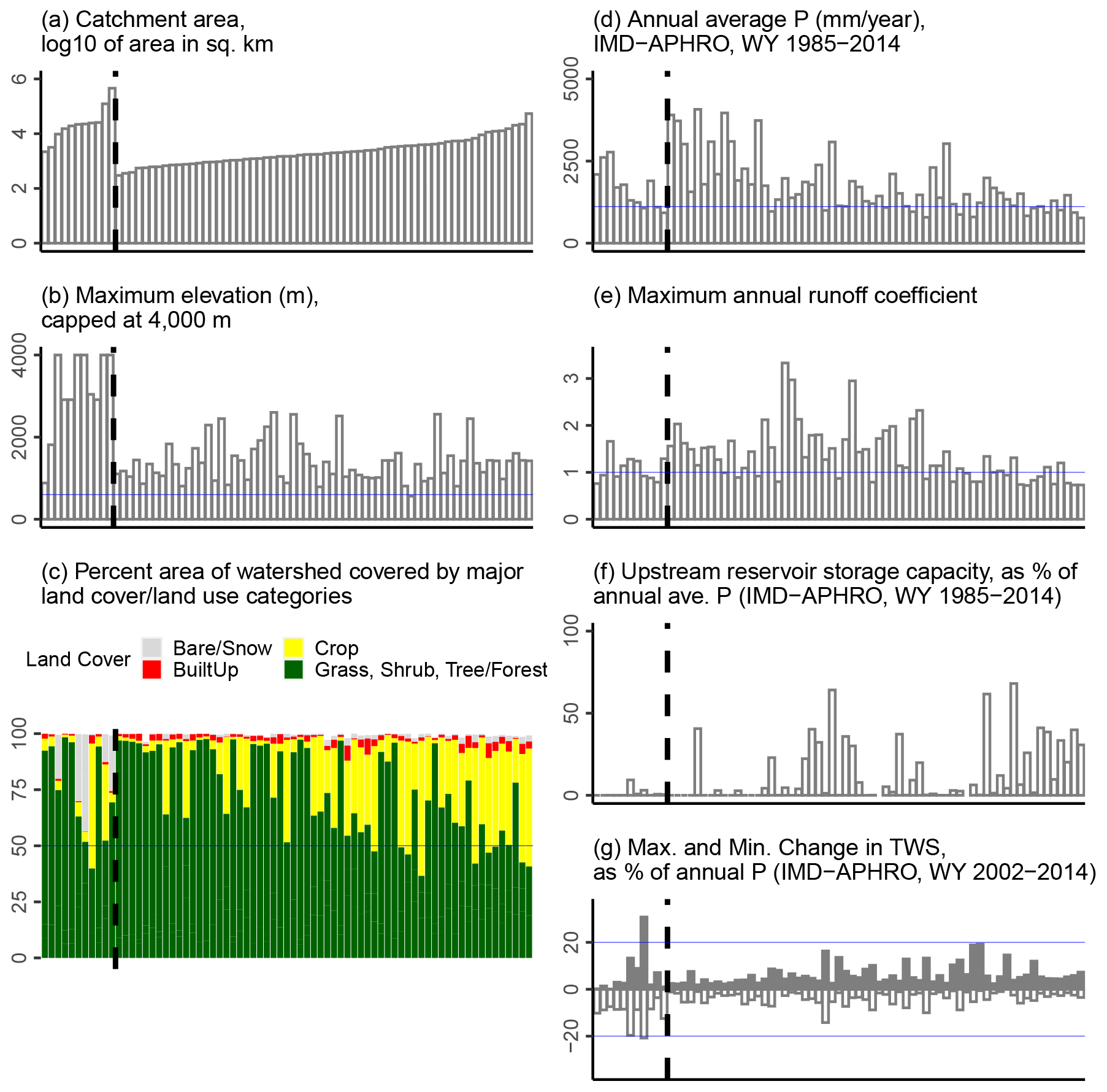
Figure 9Characteristics of the imbalanced watersheds identified using IMD-APHRO. The watersheds are sorted in ascending order of catchment area (left to right) in all of the panels. The thick broken vertical line in each plot separates the watersheds of Northern India from those of Peninsular India. (a) Catchment area; (b) maximum elevation (blue line shows the average elevation for the whole of India: 600 m); (c) land-cover and land-use fractions (blue line shows the 50 % fraction for reference); (d) average annual P (blue line shows the average annual P for the whole of India: 1100 mm); (e) maximum runoff coefficient (blue line indicates a value of 1.0); (f) cumulative maximum live storage capacity expressed as a fraction of the annual P; and (g) maximum (shaded bars) and minimum (unshaded bars) ΔTWS as fractions of the annual P.
The average annual P for these imbalanced watersheds is typically around 2000 mm yr−1 (Fig. 9d) – about twice the average annual P for the whole of India (about 1100 mm, see Table S3.1). Thus, such watersheds are typically wetter than the rest of India. Moreover, what is presented here is the observed P, which is potentially affected by UoP, and the actual P could be much higher. The maximum annual runoff coefficient for these watersheds typically exceeds 1 (median value of 1.15; maximum value of 3.33; Fig. 9e). The extent of reservoir storage is quantified as the cumulative sum of the maximum live storage capacity of all reservoirs present in the watershed, expressed as a percentage of the average annual P (Fig. 9f). While most watersheds have relatively minimal storage, some of them could have more than 50 % of the annual P captured in the reservoirs. However, the P data used here is the observed P (affected by UoP), not the actual P. Therefore, the actual effect of reservoirs is expected to be smaller than what is represented here. Finally, the minimum and maximum watershed-averaged values of ΔTWS expressed as fractions of the annual P (Fig. 9g) indicate that the magnitude of ΔTWS is less than 20 % for most of these watersheds.
Based on these physical characteristics, the imbalanced watersheds identified using the IMD-APHRO dataset are typically forested (or minimally impacted by agriculture) and located in relatively wet regions and at relatively high elevations, often have annual runoff coefficients exceeding 1.0, and, in general, are minimally impacted by reservoir storage. Moreover, based on a visual comparison of the extent of large-scale management shown in Fig. 3 and the locations of imbalanced watersheds in Fig. 8, the imbalanced watersheds can be considered to be minimally affected by groundwater extraction and diversions. Furthermore, based on a visual comparison of annual ΔTWS in Fig. 4 and the locations of imbalanced watersheds in Fig. 8, the imbalanced watersheds are typically in regions not affected by relatively large annual changes in TWS.
4.3 UoP within IMD-APHRO versus other datasets
Similar to the earlier analysis in which watersheds potentially affected by UoP were identified using the IMD-APHRO dataset, the potential UoP within other P datasets is analyzed in this section. For each P dataset, Table 3 shows the number of station-years across all imbalanced watersheds according to that dataset. The number of station-years by scenario are tabulated separately for the watersheds of Northern India and Peninsular India. Since the different P datasets have differing time spans, the total number of WYs varies by P dataset. ERA5, IMD-APHRO and TERRA have the longest time spans (782 station-years in Northern India and 6153 station-years in Peninsular India), while SM2RAIN has the shortest time span (195 station-years in Northern India and 1784 station-years in Peninsular India).
Table 3Total number of station-years analyzed and the imbalanced station-years by scenario for all the watersheds of Northern India (left) and Peninsular India (right) for each P dataset.
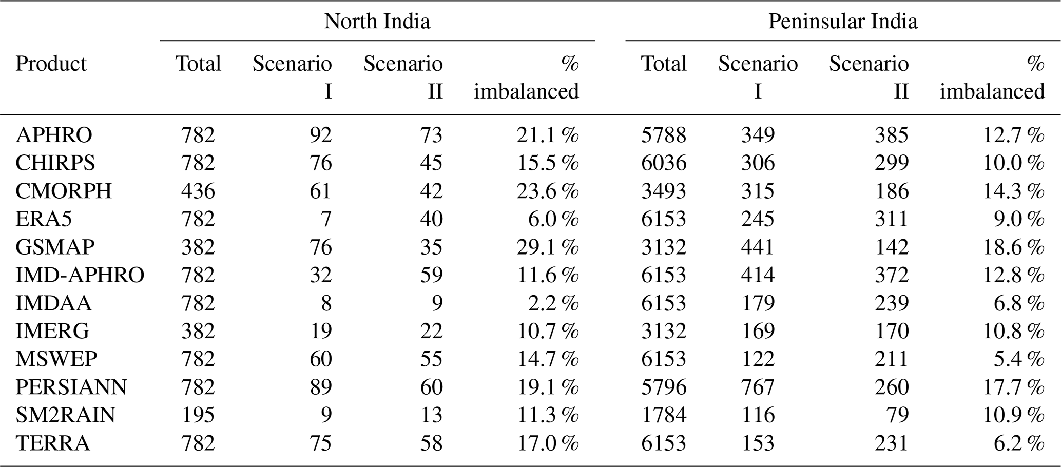
The total number of imbalanced years for which either UoP scenario is realized is expressed as the percentage of the total analyzed station-years. This percentage acts as proxy for the extent of UoP, and can vary from about 2 % to 29 % in Northern India and from 5 % to 19 % in Peninsular India, depending on the P dataset. The APHRO dataset is consistent with IMD-APHRO in Peninsular India but not in Northern India. Across the entire study domain, the satellite-based GSMAP, PERSIANN and CMORPH datasets typically have the highest percentages of imbalanced station-years, while the reanalysis-based datasets of ERA5 and IMDAA have the lowest percentages. While ERA5 and IMDAA are consistent across both Northern and Peninsular India, the MSWEP and TERRA datasets have the lowest percentages in Peninsular India but do not have such low percentages in Northern India. The reanalysis-based datasets of ERA5 and IMDAA outperform IMD-APHRO as well as the high-resolution satellite products such as CMORPH and PERSIANN. The GSMAP dataset has the highest percentage of imbalanced watersheds in both Northern and Peninsular India.
The statistics presented in Table 3 are based on a specific set of heuristics (0.70 and 1.20) used within Scenario II. In order to understand the impacts of changing the heuristics, three other sets of heuristics were tried. Instead of 0.70, values of 0.60, 0.80 and 0.90 were used, and instead of 1.20, values of 1.10, 1.30 and 1.40 were used within Scenario II. Tables S9.1–9.3 show the new set of statistics (similar to Table 3) for each set of heuristics. It is evident from these tables that the performance of the datasets remains similar to that shown in Table 3. ERA5 and IMDAA outperform IMD-APHRO consistently across both Northern and Peninsular India, while the MSWEP and TERRA datasets have the lowest percentages in Peninsular India but do not have such low percentages in Northern India.
The metrics presented in Table 3 are associated with watersheds where adequate hydrometeorological data are available. Since these watersheds are limited to only certain portions of India, these metrics do not accurately reflect the spatial distribution of UoP present within each P dataset. In order to assess the spatial distribution of UoP, potential correction factors (CFs) are estimated for select datasets in Sect. 4.4. The ERA5, IMDAA, MSWEP and TERRA datasets are chosen for further analysis because of their potential ability to be less affected by UoP than IMD-APHRO.
4.4 Potential correction factors (CFs) for specific datasets
Correction factors (CFs) represent ratios of actual and observed P. Since it is not possible to estimate them without knowing the actual P, they were estimated assuming that select datasets from the above analysis are reasonable proxies for the actual P. These estimated CFs are referred to as potential CFs to distinguish them from true CFs. As mentioned in Sect. 4.3, the ERA5, IMDAA, MSWEP and TERRA datasets suffer less from UoP than IMD-APHRO. Using these datasets, potential CFs were estimated using Eq. (7):
For each dataset, data were first aggregated to IMD's resolution of 0.25° (∼25 km). Then, for the 30-year common data period of WY 1985–2014, the gridwise average annual P was estimated. The ratio of gridwise 30-year average annual P between each dataset and IMD is presented in Fig. 10. The spatial domain is limited to the political boundaries of India where IMD data are available.
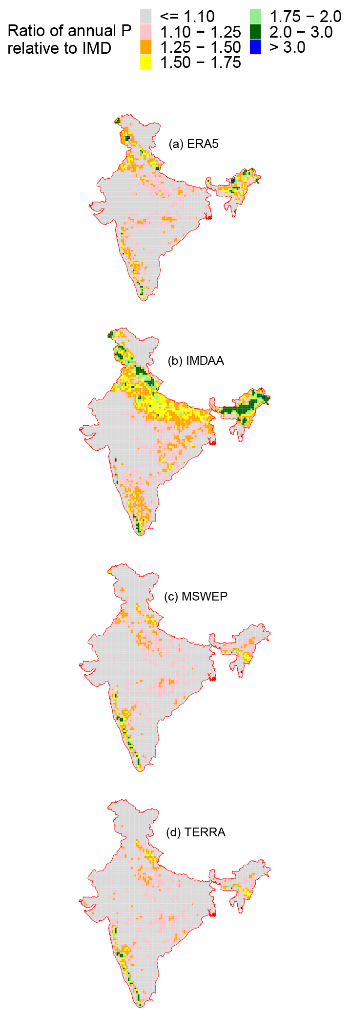
Figure 10Gridwise potential CFs for select datasets based on the period WY 1985–2014.
The spatial maps of potential CFs shown in Fig. 10 can be compared to those presented in Figs. S1.1 and S1.2. High CFs are present in the mountainous western coast of India for all four datasets and in the mountainous parts of Northern India for only fERA5 and IMDAA. This is consistent with the percentage of imbalanced station-years associated with each of these datasets (see Table 3). Another feature that is evident from Fig. 10 is that the highest CFs occur in the wettest parts of India (Fig. S1.2). If these potential CFs are reasonably accurate, then one could conclude that UoP is a substantial problem in the wettest parts of India. A CF of at least 1.5 (yellow-, green- or blue-shaded areas in Fig. 10) indicates that the actual P is at least 50 % higher than the observed P. There are wide swaths of mountainous and hilly regions of India with such CFs. In order to identify the river basins of India that are most affected by UoP, basin-aggregated potential CFs are analyzed.
Table 4Basin-aggregated potential CFs for select datasets based on the period WY 1985–2014. Average and maximum values for each dataset are shown for each river basin. The upper half of the table shows the basins of Northern India, while the lower half shows the basins of Peninsular India.
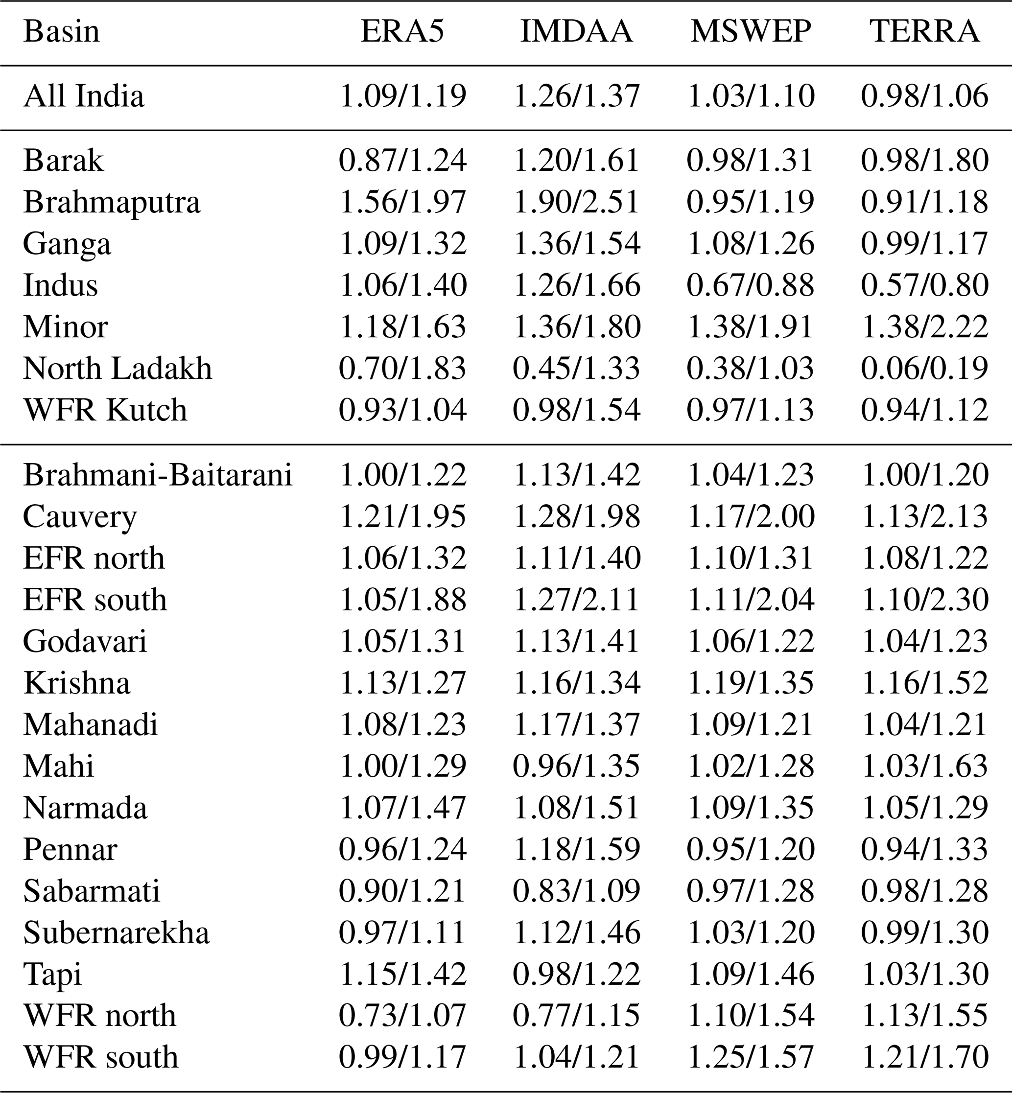
Table 4 shows the basin-aggregated potential CFs for the above four P datasets. An additional table for all of the P datasets analyzed here is shown in Table S3.1. The potential CFs shown here were estimated as the ratio of annual P for each dataset and IMD. The average and maximum values for the 30-year period of WY 1985–2014 are shown in Table 4. Since IMD is the main P dataset of interest and is limited to the political boundaries of India, only that portion of each river basin falling within India's boundaries was included when estimating these potential CFs.
Across the whole of India, ERA5, IMDAA and MSWEP are on average 9 %, 26 % and 3 % higher than IMD, respectively, while TERRA is 2 % lower than IMD. However, the maximum values indicate that ERA5, IMDAA, MSWEP and TERRA can be up to 19 %, 37 %, 10 % and 6 % higher than IMD, respectively. There is substantial variability across basins and datasets. For instance, for the Brahmaputra Basin, ERA5 and IMDAA are 56 % and 90 % higher than IMD; however, MSWEP and TERRA are 5 % and 9 % lower than IMD. Similarly, for the Ganga Basin, on average, ERA5, IMDAA and MSWEP are 9 %, 36 % and 8 % higher than IMD; however, TERRA is 1 % lower than IMD. Similarly, for the Indus Basin, on average, ERA5 and IMDAA are 6 % and 26 % higher than IMD; however, MSWEP and TERRA are 33 % and 43 % lower than IMD. This pattern of ERA5 and IMDAA being higher than IMD while MSWEP and TERRA were lower than IMD in the basins of Northern India is consistent with the potential CFs shown in Fig. 10. ERA5 and IMDAA have CFs exceeding 1 in many regions of Northern India, while MSWEP and TERRA do not have such high CFs to the same extent.
Table 4 also shows that for most basins of Peninsular India, potential CFs from the four selected P datasets are almost always greater than 1. This implies that P is underestimated across most of Peninsular India, regardless of which of the four datasets is used as a proxy for actual P. The Godavari and Krishna basins are the two largest basins of Peninsular India. In the Godavari Basin, on average, the four datasets are 4 % to 13 % higher than IMD. In the Krishna Basin, on average, the four datasets are 13 % to 19 % higher than IMD. The wettest basins of Peninsular India are the WFR north and WFR south basins. In these two basins, MSWEP and TERRA are higher than IMD, while ERA5 and IMDAA tend to be similar to or lower than IMD. This is consistent with the percentage of imbalanced station-years associated with each of these datasets in Peninsular India (see Table 3).
5.1 Limitations
The watersheds affected by UoP were identified by analyzing the extent of the annual water imbalance. As such, the results are dependent on the quality of the data and strength of the assumptions used. The limitations of the datasets used here and also the limitations imposed by the assumptions made within this analysis are discussed here.
5.1.1 Limitations of the data
The GHI dataset (Goteti, 2023) was chosen here because of the quality-controlled nature of the catchment boundaries and R data used in its development. The GHI stations used here were those that had a catchment area discrepancy of less than 5 % when compared with CWC. It is assumed that the catchment boundaries used here are reasonably accurate, and any errors in such boundaries and are not likely to cause the identified water imbalance.
GHI is limited to Peninsular India, and R data for Northern India was compiled from CWC-19 (2019). Such annual and monthly R data were compiled from daily records which are known to have missing days. Hence, the actual R is very likely higher than the observed R. Thus, it is expected that there would be more imbalanced station-years. Moreover, as additional R data from other gauging stations become available, particularly in the mountainous portions of Northern India, many other watersheds affected by UoP will be identified. All of the R data used here are directly or indirectly from the CWC. Studies have reported that R based on rating curves could have significant errors (e.g., Di Baldassarre and Montanari, 2009; Kiang et al., 2018). Huang et al. (2023) estimate that about 70 % of the global streamflow gauging stations analyzed in their study have a bias in catchment discharge of greater than 10 %. None of the stations from Huang et al. (2023) are present within this study's analysis domain. It is not known to what extent R from the CWC is derived from rating curves, to what extent such data are affected by measurement or other errors, or to what extent errors in streamflow measurement affect the streamflow data used in this analysis.
GLEAM was used as the source of ET instead of NTSG. While there is reasonable correlation between the two products, GLEAM-based ET is generally lower than NTSG-based ET (Sect. S4). Goroshi et al. (2017) indicated that NTSG underestimates lysimeter-based ET observations across many locations in India. This would imply that GLEAM would further underestimate such ET observations. Thus, ET from GLEAM should be considered a lower bound for ET. If more accurate ET estimates were to become available, it is expected that there would be more imbalanced station-years.
Management of water, such as groundwater extraction, reservoir storage and water diversion (imports or exports), is shown to be relatively minimal in the imbalanced watersheds (relative to annual P). Extent of groundwater extraction is available at district resolution and only for select years. Some studies have urged caution when interpreting trends in groundwater levels from CGWB (e.g., Hora et al., 2019). The quantification of groundwater storage in the study domain is particularly challenging due to varying geological settings (alluvial versus hard-rock aquifers), extensive and unregulated withdrawal for irrigation use, and changing energy policies (Panda et al., 2022). The dams considered here were only from India and included only the large dams available via the NRLD inventory. It is possible that smaller, or other, dams that are present in the watershed and not included within NRLD could be causing some of the water imbalance. Data on water diversions are available only for select sub-basins of the major basins of India. There are also a number of local watershed development projects that are being pursued in the forested and mountainous regions of India, such as those reported by Chauhan (2010). The effect of such development on the hydrologic budgets of the watersheds analyzed here is unknown.
GRACE-based annual changes in ΔTWS are useful for understanding the effect of such changes on the annual water budget. As discussed by Humphrey et al. (2023), numerous assumptions went into the processing of raw GRACE data, and one has to exercise caution when interpreting the end products derived from raw data. The effective resolution of GRACE is about 300 km × 300 km. Thus, watershed-scale annual ΔTWS values for the imbalanced watersheds in Fig. 9 are representative of coarser-scale patterns and complement the data on watershed management summarized in Fig. 3. GRACE-based ΔTWS cannot be directly compared to changes in the local water table. Some recent studies have assimilated GRACE observations into hydrological models to better capture finer-scale groundwater storage changes (Li et al., 2019). The use of ΔTWS from such studies could be explored in future work.
The accuracy of gauge-based products such as IMD is dependent on the underlying gauge data as well as the specific interpolation procedures used to create the gridded data. If raw gauge data are available, it might be worthwhile to compare such data with the other P datasets for select high-intensity storms in the imbalanced watersheds. The reader is referred to the studies of Prakash et al. (2015a, 2019) for information on how such comparisons could be made and also on the challenges involved in creating gridded products.
5.1.2 Limitations of the methodology
Watershed boundaries do not always coincide with underlying aquifer boundaries (e.g., Liu et al., 2020), and so one cannot always assume that water flowing out of a watershed is completely generated within the watershed. A number of studies have discussed the important role of inter-watershed groundwater flow (IGF) (e.g., Fan, 2019), including that within high mountain environments such as the Brahmaputra Basin (e.g., Somers and McKenzie, 2020; Yao et al., 2021). The contribution of IGF to the streamflow depends on a number of factors such as the geology, topography and climate, among others. While some studies have identified that karst aquifers are present in select parts of India (Dar et al., 2014), extensive watershed-specific hydrogeologic field investigations are needed (such as those by Yao et al., 2021) to quantify the effect of IGF on the streamflow. IGF is assumed to be negligible. It is possible that some or all of the watersheds analyzed here are affected by IGF. However, one should not assume that all instances of an observed annual water imbalance are solely due to IGF. As discussed in Sect. S8, there are watersheds within the study domain where it appears that IGF is unlikely to be the cause of the observed water imbalance.
Yao et al. (2021) analyzed the contribution of groundwater to R in the upper reaches of the Brahmaputra Basin. Several watersheds from the study of Yao et al. (2021) had annual runoff coefficients greater than 1 due to a contribution from IGF as well as snowmelt and permafrost thawing. The contribution of seasonal snow melt is implicitly considered within the observed R, but glacier melt has not been considered. In the Himalayan mountains, glacier melt could sometimes be a significant portion of the annual runoff and could even exceed snow melt (e.g., Mukhopadhyay and Khan, 2015). In such watersheds where glacier melt is substantial, the annual observed R could be higher than the annual P, despite there being no management. The GRACE-based ΔTWS is supposed to capture storage changes due to glacier melt at the spatial scale of major river basins but not across smaller watersheds. It is possible that the approach adopted here could incorrectly identify such watersheds as being affected by UoP.
The identification of watersheds affected by UoP focuses on those regions where there is a relatively minimal effect of management or where the annual ΔTWS is minimal relative to P. It is not clear how to identify UoP when there is moderate to extensive management or annual ΔTWS is substantial relative to P. Analyzing the relative magnitudes of the individual terms of the water budget might not be the way to identify UoP under such circumstances. The two water imbalance scenarios investigated here are only two of the many possible scenarios. The imbalanced watersheds identified here are dependent on the formulation of such scenarios.
The formulation of Scenarios I and II relies more on R and less on ET. This is because, while observations of R are available, the observed ET at the scale of the watersheds analyzed here is non-existent. Satellite-based ET was used as a proxy for observed ET. However, such ET data can have substantial biases (e.g., Goroshi et al., 2017; Goteti, 2022). Hence, observed R is assumed to be more reliable than satellite-based ET. If one had more reliable estimates of ET, then the formulation of the scenarios could be revised to include other instances of a spurious water imbalance.
5.2 Spurious patterns within IMD
During the course of this analysis, several potential issues with trends in the IMD dataset were encountered. The following is a discussion on basin-scale trends in the IMD dataset and those present in other datasets. For the purposes of this discussion, the spatial domain is limited to the political boundaries of India where IMD data are available. Basin-scale aggregation of gridded P was performed only using the grids within India's boundaries.
Trends in the four datasets identified in Sect. 4.3 are compared against those in IMD. Trends in basin-aggregated annual P for WY 1985–2014 were estimated using the non-parametric Theil–Sen slope (Helsel et al., 2020), making use of the R statistical package “RobustLinearReg” (Hurtado, 2023). Table 5 shows the trends for select basins where mountains are present. Table S3.2 shows the trends for all of the basins and all of the P datasets.
Table 5Trends in annual basin-aggregated P (mm yr−1) for WY 1985–2014 for select datasets and select river basins. Values that are statistically significant at the 95 % confidence level are indicated by *.
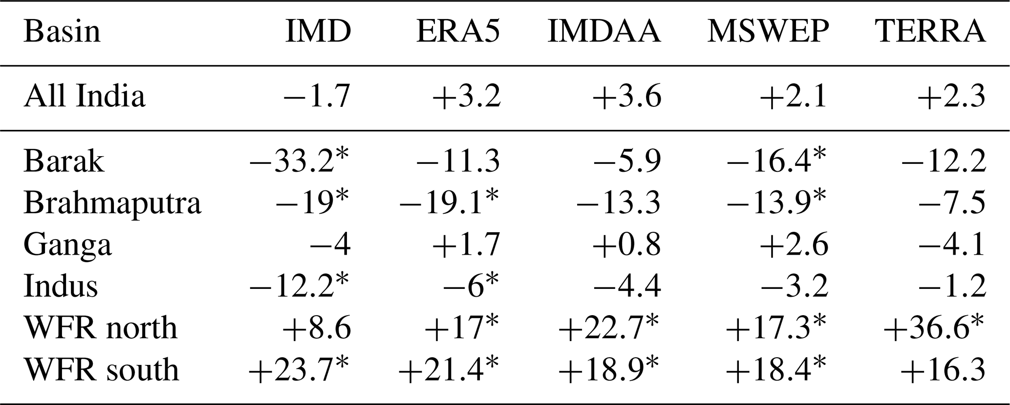
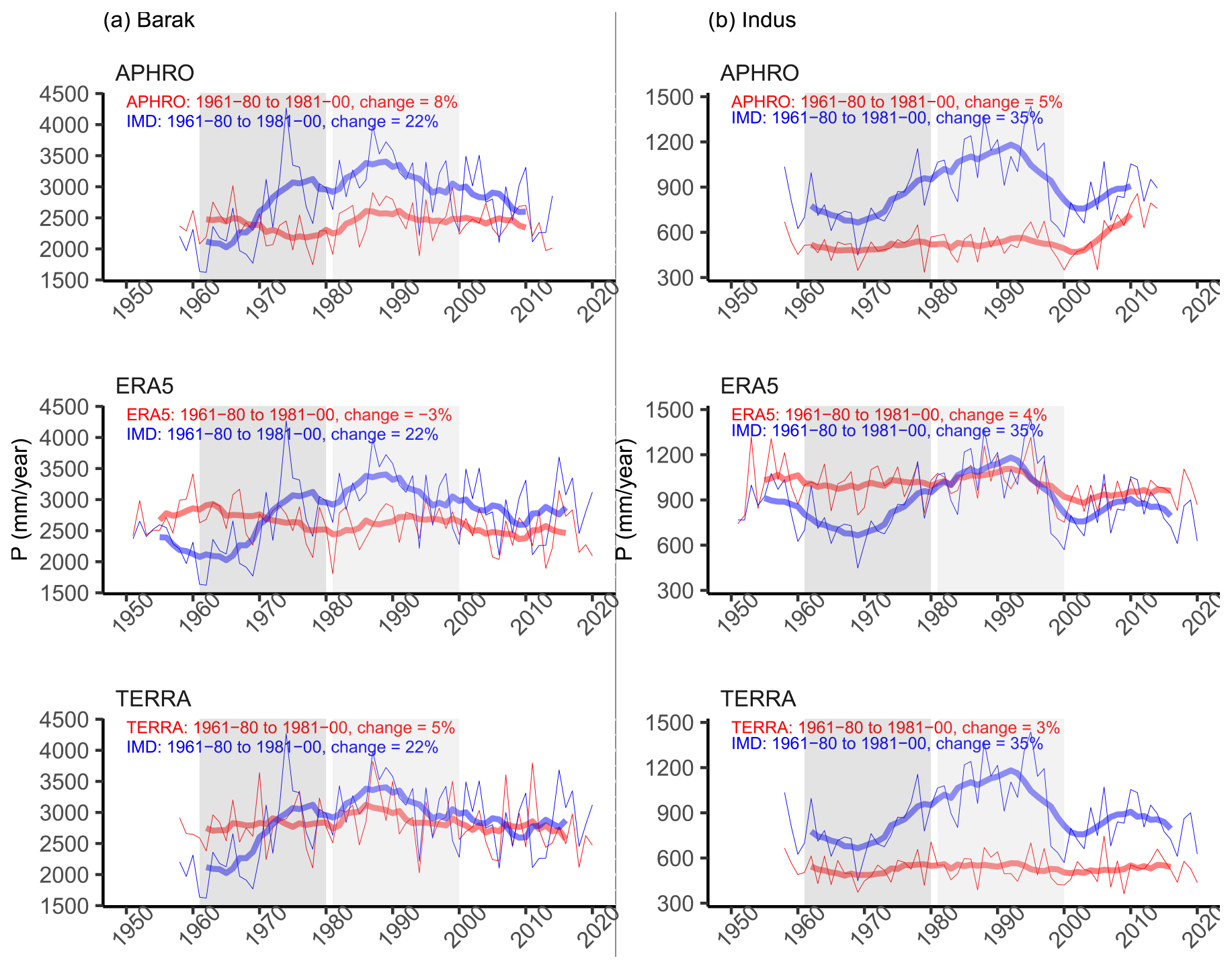
Figure 11(a) Annual P for Barak Basin for select datasets. IMD (blue) is compared against select datasets. The periods of interest, WY 1961–1980 and WY 1981–2000, are highlighted. Thin lines show the annual values, while the thick lines show the 9-year running average. (b) Same as (a) but for the Indus Basin.
The annual P from IMD for the whole of India shows a decreasing trend of −1.7 mm yr−1. In contrast to IMD's decreasing trend, all other datasets have an increasing trend. However, none of these trends are statistically significant at the 95 % confidence level. There is substantial variation in regional trends, as is evident in the trends presented for individual basins. For the IMD dataset, the Barak, Brahmaputra, Ganga and Indus basins in Northern India show decreasing trends. However, other datasets do not always have the same magnitude or sign as IMD. For instance, for the Ganga Basin, IMD shows a negative trend of −4 mm yr−1, while ERA5, IMDAA and MSWEP show a positive trend. None of these trends are statistically significant at the 95 % confidence level. For the wettest basin of India, the WFR south basin, all datasets show a positive trend, with most of them being statistically significant. Based on Table S3.2, there appears to be more consistency in trends between IMD and other datasets for the basins of Peninsular India compared to the basins of Northern India.
Another issue which was encountered was abrupt changes in the time series of P from the IMD dataset, particularly in the earlier part of its record. The time period of interest here is the 20-year period of WY 1981–2000, which is compared to the prior 20-year period of WY 1961–1980. The time series of basin-averaged annual P from IMD is compared with the corresponding time series from three P datasets which have data available for these periods – APHRO (gauge-based), ERA5 and TERRA (reanalysis-based).
Figure 11 shows such comparisons for the Barak and Indus basins, while Figs. S3.16 to S3.38 show a similar time series comparison for all of the major basins. Both annual values (thin lines) and the 9-year running average (thick lines) are shown in Fig. 11 to highlight the short- and long-term changes in P in each of the datasets. Figure 11 shows that for the Barak Basin, IMD shows an increase in average annual P of about 22 % for WY 1981–2000 relative to WY 1961–1980. However, APHRO, ERA5 and TERRA show a change of 8 %, −3 % and 5 %, respectively. Also, IMD has a distinct visual increasing trend from low values in the early 1960s to high values in the early 1990s. Such a pattern is not present in APHRO, ERA5 or TERRA. Similarly, for the Indus Basin, IMD shows an increase in average annual P of about 35 % for WY 1981–2000 relative to WY 1961–1980. However, APHRO, ERA5 and TERRA show a change of 5 %, 4 % and 3 %, respectively. IMD, once again, has a distinct visual increasing trend from low values in the mid 1970s to high values in the late 1990s. Such a pattern is not present in APHRO, ERA5 or TERRA.
Overall, the above discussion highlights two related issues with the IMD dataset. First, trends present within the IMD dataset are not always present in other datasets. Second, the conspicuous temporal shifts present in the IMD dataset are not present in other datasets. Lin and Huybers (2019) noted a potentially spurious shift in the IMD dataset over central India. It is not known if, and to what extent, such issues are caused by UoP within these datasets.
5.3 Interim measures
Solving the problem of UoP by increasing the station density in relevant areas, by monitoring and analyzing extreme P events and rainfall–runoff relationships for such events, or by any other means requires significant planning and resources from the relevant government agencies. Such efforts are strongly encouraged by the authors. In the interim, there are several useful and feasible ideas the community could pursue to help address the issue of UoP. The following is a brief discussion of such ideas.
Raw station data from the IMD would be extremely helpful for resolving discrepancies associated with trends and discrepancies with other datasets. However, such data are not publicly available. The IMD could help resolve the issue of UoP by making such raw station data publicly available. Other data from India's water agencies, such as streamflow data, which are currently classified by the CWC for Northern India, would also be valuable for addressing UoP.
Some studies have demonstrated the ability of high-resolution simulation models to capture P in watersheds dominated by hilly or mountainous terrain. For instance, Li et al. (2017) implemented the Weather Research and Forecasting (WRF) Hydro model in a high-resolution setting (3 km grid) across a mountainous watershed of Northern India. They demonstrated that such a system can reasonably simulate P and can overcome the deficiencies of typical gauge-based products and satellite-based products. Hunt and Menon (2020) also used the WRF-Hydro modeling system in a high-resolution setting (4 km grid) to analyze P during the catastrophic flooding of 2018 in the state of Kerala in Peninsular India. Their study was also able to capture the spatial structure and magnitude of the observed P reasonably well. Such modeling studies should be pursued further to better identify and quantify UoP within traditional products.
The gross underestimation of precipitation (UoP) in India was analyzed using a water balance approach across 242 watersheds of Northern and Peninsular India. Gross UoP was identified by comparing the water year (WY)-based volume of observed annual P against the observed annual streamflow (R) and comparing P against the sum of R and satellite-based evapotranspiration (ET). Across many watersheds of both Northern and Peninsular India, the spurious water imbalance scenarios of P≤R oder were realized. It was shown that the occurrence of such imbalances is unlikely to be due to the large-scale management of water, such as groundwater extraction, reservoir storage and diversions. It was also shown that the occurrence of such imbalances is unlikely to be due to annual changes in terrestrial water storage. Assuming that the data on R and ET are reliable, it was concluded that UoP is the likely cause of such spurious imbalances. The effect of the inter-watershed groundwater flow has been ignored. However, it appears that such groundwater flow is unlikely to be the cause of the spurious water imbalances observed in some of the watersheds.
All 12 state-of-the-art P products analyzed here suffer from UoP but to a varying extent. Within the often-used IMD dataset, UoP is an issue in most major river basins of India and is present throughout the historical record, including the decade of the 2010s. Based on the limited observation data available, UoP is found typically in the relatively wet regions of India. Thus, our understanding of the hydrology of India is limited by inadequate P data, particularly in these wet regions, some of which have experienced catastrophic flooding in recent years. Moreover, the P product from IMD, which is typically the benchmark in many hydrological and environmental studies across India, suffers from UoP more than some products based on reanalysis. The P from such products tends to be much higher than IMD across most river basins of India. Furthermore, such products do not have the spurious temporal patterns found in IMD. Studies using the IMD dataset should exercise caution, particularly in regions with hilly or mountainous terrain. This study highlights not only a major limitation of existing P products over India but also other data-related obstacles faced by the research community.
The supplementary material has additional graphics and summary tables that are relevant to the paper. Data files included with the Supplement contain metadata on gauging stations, GIS data on catchment boundaries, GIS data on river basin boundaries and time series of the hydrometeorological data associated with each station (see Sect. S2).
The supplement related to this article is available online at: https://doi.org/10.5194/hess-28-3435-2024-supplement.
GG and JF collaborated on the conceptual framework of the analysis and the writing of the paper. GG performed the analyses.
The contact author has declared that neither of the authors has any competing interests.
Publisher's note: Copernicus Publications remains neutral with regard to jurisdictional claims made in the text, published maps, institutional affiliations, or any other geographical representation in this paper. While Copernicus Publications makes every effort to include appropriate place names, the final responsibility lies with the authors.
The software used here includes the R statistical computing and graphics software for data analysis (https://www.r-project.org/, R Foundation, 2024) and QGIS for GIS analysis (https://qgis.org/en/site/, QGIS, 2024). Political boundaries for India were obtained from the Survey of India (https://surveyofindia.gov.in/, Survey of India, 2024). The authors would like to thank the editor and the reviewers for their help improving the original manuscript.
This paper was edited by Nadav Peleg and reviewed by Namendra Kumar Shahi and one anonymous referee.
Abatzoglou, J. T., Dobrowski, S. Z., Parks, S. A., and Hegewisch, K. C.: TerraClimate, a high-resolution global dataset of monthly climate and climatic water balance from 1958–2015, Sci. Data, 5, 1–12, https://doi.org/10.1038/sdata.2017.191, 2018. a
Adam, J. C. and Lettenmaier, D. P.: Adjustment of global gridded precipitation for systematic bias, J. Geophys. Res.-Atmos., 108, 4257, https://doi.org/10.1029/2002JD002499, 2003. a
Adam, J. C., Clark, E. A., Lettenmaier, D. P., and Wood, E. F.: Correction of global precipitation products for orographic effects, J. Climate, 19, 15–38, https://doi.org/10.1175/JCLI3604.1, 2006. a
Beck, H. E., Wood, E. F., Pan, M., Fisher, C. K., Miralles, D. G., Van Dijk, A. I., McVicar, T. R., and Adler, R. F.: MSWEP V2 global 3-hourly 0.1 precipitation: methodology and quantitative assessment, B. Am. Meteorol. Soc., 100, 473–500, https://doi.org/10.1175/BAMS-D-17-0138.1, 2019. a
Beck, H. E., Wood, E. F., McVicar, T. R., Zambrano-Bigiarini, M., Alvarez-Garreton, C., Baez-Villanueva, O. M., Sheffield, J., and Karger, D. N.: Bias correction of global high-resolution precipitation climatologies using streamflow observations from 9372 catchments, J. Climate, 33, 1299–1315, https://doi.org/10.1175/JCLI-D-19-0332.1, 2020. a, b, c
Brocca, L., Filippucci, P., Hahn, S., Ciabatta, L., Massari, C., Camici, S., Schüller, L., Bojkov, B., and Wagner, W.: SM2RAIN–ASCAT (2007–2018): global daily satellite rainfall data from ASCAT soil moisture observations, Earth Syst. Sci. Data, 11, 1583–1601, https://doi.org/10.5194/essd-11-1583-2019, 2019. a
Buchhorn, M., Smets, B., Bertels, L., De Roo, B., Lesiv, M., Tsendbazar, N.-E., Herold, M., and Fritz, S.: Copernicus global land service: Land cover 100 m: collection 3: epoch 2019: Globe, Version V3.0.1, Zenodo [data set], https://doi.org/10.5281/zenodo.3939050, 2020. a
Chauhan, B. S., Kaur, P., Mahajan, G., Randhawa, R. K., Singh, H., and Kang, M. S.: Global warming and its possible impact on agriculture in India, Adv. Agron., 123, 65–121, https://doi.org/10.1016/B978-0-12-420225-2.00002-9, 2014. a
Chauhan, M.: A perspective on watershed development in the Central Himalayan State of Uttarakhand, India, Int. J. Ecol. Environ. Sci., 36, 253–269, 2010. a
CWC-19: Reassessment of Water Availability in India using Space Inputs, Central Water Commission, Basin Planning and Management Organisation, http://www.cwc.gov.in/water-resource-estimation (last access: 15 January 2024), 2019. a, b, c, d, e, f, g, h
Dahri, Z. H., Moors, E., Ludwig, F., Ahmad, S., Khan, A., Ali, I., and Kabat, P.: Adjustment of measurement errors to reconcile precipitation distribution in the high-altitude Indus basin, Int. J. Climatol., 38, 3842–3860, https://doi.org/10.1002/joc.5539, 2018. a
Dangol, S., Talchabhadel, R., and Pandey, V. P.: Performance evaluation and bias correction of gridded precipitation products over Arun River Basin in Nepal for hydrological applications, Theor. Appl. Climatol., 148, 1353–1372, https://doi.org/10.1007/s00704-022-04001-y, 2022. a
Dar, F. A., Perrin, J., Ahmed, S., and Narayana, A. C.: Carbonate aquifers and future perspectives of karst hydrogeology in India, Hydrogeol. J., 22, 1493, https://doi.org/10.1007/s10040-014-1151-z, 2014. a
Di Baldassarre, G. and Montanari, A.: Uncertainty in river discharge observations: a quantitative analysis, Hydrol. Earth Syst. Sci., 13, 913–921, https://doi.org/10.5194/hess-13-913-2009, 2009. a
Famiglietti, J. S.: The global groundwater crisis, Nat. Clim. Change, 4, 945–948, https://doi.org/10.1038/nclimate2425, 2014. a
Fan, Y.: Are catchments leaky?, Wiley Interdisciplin. Rev.: Water, 6, e1386, https://doi.org/10.1002/wat2.1386, 2019. a, b
Funk, C. C., Peterson, P. J., Landsfeld, M. F., Pedreros, D. H., Verdin, J. P., Rowland, J. D., Romero, B. E., Husak, G. J., Michaelsen, J. C., and Verdin, A. P.: A quasi-global precipitation time series for drought monitoring, US Geological Survey data series 832, 1–12, US Geological Survey, https://doi.org/10.3133/ds832, 2014. a
Goroshi, S., Pradhan, R., Singh, R. P., Singh, K., and Parihar, J. S.: Trend analysis of evapotranspiration over India: Observed from long-term satellite measurements, J. Earth Syst. Sci., 126, 1–21, https://doi.org/10.1007/s12040-017-0891-2, 2017. a, b
Goteti, G.: Estimation of water resources availability (WRA) using gridded evapotranspiration data: A simpler alternative to Central Water Commission's WRA assessment, J. Earth Syst. Sci., 131, 1–24, 2022. a
Goteti, G.: Geospatial dataset for hydrologic analyses in India (GHI): a quality-controlled dataset on river gauges, catchment boundaries and hydrometeorological time series, Earth Syst. Sci. Data, 15, 4389–4415, https://doi.org/10.5194/essd-15-4389-2023, 2023. a, b, c, d
Gupta, P., Chauhan, S., and Oza, M.: Modelling surface run-off and trends analysis over India, J. Earth Syst. Sci., 125, 1089–1102, https://doi.org/10.1007/s12040-016-0720-z, 2016. a
Gupta, V., Jain, M. K., Singh, P. K., and Singh, V.: An assessment of global satellite-based precipitation datasets in capturing precipitation extremes: A comparison with observed precipitation dataset in India, Int. J. Climatol., 40, 3667–3688, https://doi.org/10.1002/joc.6419, 2020. a
Helsel, D. R., Hirsch, R. M., Ryberg, K. R., Archfield, S. A., and Gilroy, E. J.: Statistical methods in water resources: US Geological Survey Techniques and Methods, book 4, chap. A3, US Geological Survey, https://doi.org/10.3133/tm4a3, 2020. a
Hora, T., Srinivasan, V., and Basu, N. B.: The groundwater recovery paradox in South India, Geophys. Res. Lett., 46, 9602–9611, https://doi.org/10.1029/2019GL083525, 2019. a
Huang, P., Wang, G., Guo, L., Mello, C. R., Li, K., Ma, J., and Sun, S.: Most global gauging stations present biased estimations of total catchment discharge, Geophys. Res. Lett., 50, e2023GL104253, https://doi.org/10.1029/2023GL104253, 2023. a, b
Huffman, G. J., Bolvin, D. T., Braithwaite, D., Hsu, K.-L., Joyce, R. J., Kidd, C., Nelkin, E. J., Sorooshian, S., Stocker, E. F., Tan, J., Wolff, D. B., and Xie, P.: Integrated multi-satellite retrievals for the global precipitation measurement (GPM) mission (IMERG), Satellite Precipitation Measurement: Volume 1, 343–353, Springer, https://doi.org/10.1007/978-3-030-24568-9_19, 2020. a
Humphrey, V., Rodell, M., and Eicker, A.: Using satellite-based terrestrial water storage data: A review, Surv. Geophys., 44, 1489–1517, https://doi.org/10.1007/s10712-022-09754-9, 2023. a, b
Hunt, K. M. and Menon, A.: The 2018 Kerala floods: a climate change perspective, Clim. Dynam., 54, 2433–2446, https://doi.org/10.1007/s00382-020-05123-7, 2020. a, b
Hurtado, S.: RobustLinearReg: Robust Linear Regressions, R package version 1.2.0, https://cran.r-project.org/package=RobustLinearReg (last access: 15 January 2024), 2023. a
Kanda, N., Negi, H., Rishi, M. S., and Kumar, A.: Performance of various gridded temperature and precipitation datasets over Northwest Himalayan Region, Environ. Res. Commun., 2, 085002, https://doi.org/10.1088/2515-7620/ab9991, 2020. a
Kiang, J. E., Gazoorian, C., McMillan, H., Coxon, G., Le Coz, J., Westerberg, I. K., Belleville, B., Sevrez, D., Sikorska, A. E., Petersen-Øverleir, A., Reitan, T., Freer, J., Renard, B., Mansanarez, V., and Mason, R.: A comparison of methods for streamflow uncertainty estimation, Water Resour. Res., 54, 7149–7176, https://doi.org/10.1029/2018WR022708, 2018. a
King, A. D., Alexander, L. V., and Donat, M. G.: The efficacy of using gridded data to examine extreme rainfall characteristics: a case study for Australia, Int. J. Climatol., 33, 2376–2387, https://doi.org/10.1002/joc.3588, 2013. a
Kochendorfer, J., Rasmussen, R., Wolff, M., Baker, B., Hall, M. E., Meyers, T., Landolt, S., Jachcik, A., Isaksen, K., Brækkan, R., and Leeper, R.: The quantification and correction of wind-induced precipitation measurement errors, Hydrol. Earth Syst. Sci., 21, 1973–1989, https://doi.org/10.5194/hess-21-1973-2017, 2017. a
Krishnan, R., Sanjay, J., Gnanaseelan, C., Mujumdar, M., Kulkarni, A., and Chakraborty, S.: Assessment of climate change over the Indian region: a report of the ministry of earth sciences (MOES), government of India, Springer Nature, https://library.oapen.org/handle/20.500.12657/39973 (last access: 15 January 2024), 2020. a, b
Kubota, T., Aonashi, K., Ushio, T., Shige, S., Takayabu, Y. N., Kachi, M., Arai, Y., Tashima, T., Masaki, T., Kawamoto, N., Mega, T., Yamamoto, M. K., Hamada, A., Yamaji, M., Liu G., and Oki, R.: Global Satellite Mapping of Precipitation (GSMaP) products in the GPM era, Satellite Precipitation Measurement: Volume 1, Springer, 355–373, https://doi.org/10.1007/978-3-030-24568-9_20, 2020. a
Li, B., Rodell, M., Kumar, S., Beaudoing, H. K., Getirana, A., Zaitchik, B. F., Goncalves, L. G., Cossetin, C., Bhanja, S., Mukherjee, A., Tian, S., Tangdamrongsub, N., Long, D., Nanteza, J., Lee, J., Policelli, F., Goni, I. B., Daira, D., Bila, M., Lannoy, G., Mocko, D., Steele-Dunne, S. C., Save, H., and Bettadpur, S.: Global GRACE data assimilation for groundwater and drought monitoring: Advances and challenges, Water Resour. Res., 55, 7564–7586, https://doi.org/10.1029/2018WR024618, 2019. a
Li, L., Gochis, D. J., Sobolowski, S., and Mesquita, M. D.: Evaluating the present annual water budget of a Himalayan headwater river basin using a high-resolution atmosphere-hydrology model, J. Geophys. Res.-Atmos., 122, 4786–4807, https://doi.org/10.1002/2016JD026279, 2017. a, b
Lin, M. and Huybers, P.: If rain falls in India and no one reports it, are historical trends in monsoon extremes biased?, Geophys. Res. Lett., 46, 1681–1689, https://doi.org/10.1029/2018GL079709, 2019. a, b
Liu, Y., Wagener, T., Beck, H. E., and Hartmann, A.: What is the hydrologically effective area of a catchment?, Environ. Res. Lett., 15, 104024, https://doi.org/10.1088/1748-9326/aba7e5, 2020. a, b
Mahto, S. S., Nayak, M. A., Lettenmaier, D. P., and Mishra, V.: Atmospheric rivers that make landfall in India are associated with flooding, Commun. Earth Environ., 4, 120, https://doi.org/10.1038/s43247-023-00775-9, 2023. a
Martens, B., Miralles, D. G., Lievens, H., van der Schalie, R., de Jeu, R. A. M., Fernández-Prieto, D., Beck, H. E., Dorigo, W. A., and Verhoest, N. E. C.: GLEAM v3: satellite-based land evaporation and root-zone soil moisture, Geosci. Model Dev., 10, 1903–1925, https://doi.org/10.5194/gmd-10-1903-2017, 2017. a, b
Miralles, D. G., Holmes, T. R. H., De Jeu, R. A. M., Gash, J. H., Meesters, A. G. C. A., and Dolman, A. J.: Global land-surface evaporation estimated from satellite-based observations, Hydrol. Earth Syst. Sci., 15, 453–469, https://doi.org/10.5194/hess-15-453-2011, 2011. a, b
Mukhopadhyay, B. and Khan, A.: A reevaluation of the snowmelt and glacial melt in river flows within Upper Indus Basin and its significance in a changing climate, J. Hydrol., 527, 119–132, https://doi.org/10.1016/j.jhydrol.2015.04.045, 2015. a
Muñoz-Sabater, J., Dutra, E., Agustí-Panareda, A., Albergel, C., Arduini, G., Balsamo, G., Boussetta, S., Choulga, M., Harrigan, S., Hersbach, H., Martens, B., Miralles, D. G., Piles, M., Rodríguez-Fernández, N. J., Zsoter, E., Buontempo, C., and Thépaut, J.-N.: ERA5-Land: a state-of-the-art global reanalysis dataset for land applications, Earth Syst. Sci. Data, 13, 4349–4383, https://doi.org/10.5194/essd-13-4349-2021, 2021. a
NRLD: National Register of Large Dams, Central Water Commission, Central Dam Safety Organization, http://www.cwc.gov.in/publication/nrld (last access: 15 January 2024), 2019. a
Pai, D., Sridhar, L., Rajeevan, M., Sreejith, O., Satbhai, N., and Mukhopadhyay, B.: Development of a new high spatial resolution (0.25×0.25) long period (1901–2010) daily gridded rainfall data set over India and its comparison with existing data sets over the region, Mausam, 65, 1–18, 2014. a, b
Panda, D. K., Tiwari, V. M., and Rodell, M.: Groundwater variability across India, under contrasting human and natural conditions, Earth's Future, 10, e2021EF002513, https://doi.org/10.1029/2021EF002513, 2022. a
Prakash, S.: Performance assessment of CHIRPS, MSWEP, SM2RAIN-CCI, and TMPA precipitation products across India, J. Hydrol., 571, 50–59, https://doi.org/10.1016/j.jhydrol.2019.01.036, 2019. a
Prakash, S., Mitra, A. K., Momin, I. M., Pai, D., Rajagopal, E., and Basu, S.: Comparison of TMPA-3B42 versions 6 and 7 precipitation products with gauge-based data over India for the southwest monsoon period, J. Hydrometeorol., 16, 346–362, https://doi.org/10.1175/JHM-D-14-0024.1, 2015a. a
Prakash, S., Mitra, A. K., Momin, I. M., Rajagopal, E., Basu, S., Collins, M., Turner, A. G., Achuta Rao, K., and Ashok, K.: Seasonal intercomparison of observational rainfall datasets over India during the southwest monsoon season, Int. J. Climatol., 35, 2326–2338, https://doi.org/10.1002/joc.4129, 2015b. a
Prakash, S., Seshadri, A., Srinivasan, J., and Pai, D.: A new parameter to assess impact of rain gauge density on uncertainty in the estimate of monthly rainfall over India, J. Hydrometeorol., 20, 821–832, https://doi.org/10.1175/JHM-D-18-0161.1, 2019. a, b
Rana, S., McGregor, J., and Renwick, J.: Precipitation seasonality over the Indian subcontinent: An evaluation of gauge, reanalyses, and satellite retrievals, J. Hydrometeorol., 16, 631–651, https://doi.org/10.1175/JHM-D-14-0106.1, 2015. a
QGIS: Free and Open Source Spatial without Compromise, https://qgis.org/en/site/ (last access: 15 January 2024), 2024. a
Rani, S. I., Arulalan, T., George, J. P., Rajagopal, E., Renshaw, R., Maycock, A., Barker, D. M., and Rajeevan, M.: IMDAA: High-Resolution Satellite-Era Reanalysis for the Indian Monsoon Region, J. Climate, 34, 5109–5133, https://doi.org/10.1175/JCLI-D-20-0412.1, 2021. a
R Foundation: The R Project for Statistical Computing, https://www.r-project.org/ (last access: 15 January 2024), 2024. a
Rodell, M., Velicogna, I., and Famiglietti, J. S.: Satellite-based estimates of groundwater depletion in India, Nature, 460, 999–1002, https://doi.org/10.1038/nature08238, 2009. a
Sadeghi, M., Nguyen, P., Naeini, M. R., Hsu, K., Braithwaite, D., and Sorooshian, S.: PERSIANN-CCS-CDR, a 3-hourly 0.04 global precipitation climate data record for heavy precipitation studies, Sci. Data, 8, 157, https://doi.org/10.1038/s41597-021-00940-9, 2021. a
Save, H.: GCSR GRACE and GRACE-FO RL06 Mascon Solutions v02, Tech. rep., Center for Space Research, University of Texas, Austin, TX, https://doi.org/10.15781/cgq9-nh24, 2020. a
Save, H., Bettadpur, S., and Tapley, B. D.: High-resolution CSR GRACE RL05 mascons, J. Geophys. Res.-Solid, 121, 7547–7569, https://doi.org/10.1002/2016JB013007, 2016. a
Shahi, N. K.: Fidelity of the latest high-resolution CORDEX-CORE regional climate model simulations in the representation of the Indian summer monsoon precipitation characteristics, Clim. Dynam., 1–23, https://doi.org/10.1007/s00382-022-06602-9, 2022. a
Somers, L. D. and McKenzie, J. M.: A review of groundwater in high mountain environments, Wiley Interdisciplin. Rev.: Water, 7, e1475, https://doi.org/10.1002/wat2.1475, 2020. a
Sun, Q., Miao, C., Duan, Q., Ashouri, H., Sorooshian, S., and Hsu, K.-L.: A review of global precipitation data sets: Data sources, estimation, and intercomparisons, Rev. Geophys., 56, 79–107, https://doi.org/10.1002/2017RG000574, 2018. a
Survey of India: Office of the Surveyor General of India, https://surveyofindia.gov.in/ (last access: 15 January 2024), 2024. a
Tapley, B. D., Bettadpur, S., Ries, J. C., Thompson, P. F., and Watkins, M. M.: GRACE measurements of mass variability in the Earth system, Science, 305, 503–505, https://doi.org/10.1126/science.1099192, 2004. a
Thakur, M. K., Kumar, T., Koteswara Rao, K., Barbosa, H., and Rao, V. B.: A new perspective in understanding rainfall from satellites over a complex topographic region of India, Sci. Rep., 9, 1–10, https://doi.org/10.1038/s41598-019-52075-y, 2019. a
Xie, P., Joyce, R., Wu, S., Yoo, S.-H., Yarosh, Y., Sun, F., and Lin, R.: Reprocessed, bias-corrected CMORPH global high-resolution precipitation estimates from 1998, J. Hydrometeorol., 18, 1617–1641, https://doi.org/10.1175/JHM-D-16-0168.1, 2017. a
Xiong, J., Yin, J., Guo, S., He, S., Chen, J., and Abhishek, A.: Annual runoff coefficient variation in a changing environment: a global perspective, Environ. Res. Lett., 17, 064006, https://doi.org/10.1088/1748-9326/ac62ad, 2022. a
Yao, Y., Zheng, C., Andrews, C. B., Scanlon, B. R., Kuang, X., Zeng, Z., Jeong, S.-J., Lancia, M., Wu, Y., and Li, G.: Role of groundwater in sustaining northern Himalayan rivers, Geophys. Res. Lett., 48, e2020GL092354, https://doi.org/10.1029/2020GL092354, 2021. a, b, c, d
Yatagai, A., Kamiguchi, K., Arakawa, O., Hamada, A., Yasutomi, N., and Kitoh, A.: APHRODITE: Constructing a long-term daily gridded precipitation dataset for Asia based on a dense network of rain gauges, B. Am. Meteorol. Soc., 93, 1401–1415, https://doi.org/10.1175/BAMS-D-11-00122.1, 2012. a, b
Zhang, K., Kimball, J. S., Nemani, R. R., and Running, S. W.: A continuous satellite-derived global record of land surface evapotranspiration from 1983 to 2006, Water Resour. Res., 46, W09522, https://doi.org/10.1029/2009WR008800, 2010. a, b