the Creative Commons Attribution 4.0 License.
the Creative Commons Attribution 4.0 License.
 | 19 Aug 2024
Estimating velocity distribution and flood discharge at river bridges using entropy theory – insights from computational fluid dynamics flow fields
Farhad Bahmanpouri
Tommaso Lazzarin
Silvia Barbetta
Tommaso Moramarco
Estimating the flow velocity and discharge in rivers is of particular interest for monitoring, modeling, and research purposes. Instruments for measuring water level and surface velocity are generally mounted on bridge decks, and this poses a challenge because the bridge structure, with piers and abutments, can perturb the flow field. The current research aims to investigate the applicability of entropy theory to estimate the velocity distribution and the discharge in the vicinity of river bridges. For this purpose, a computational fluid dynamics (CFD) model is used to obtain three-dimensional flow fields along a stretch of the Paglia River (central Italy), where a historical multi-arch bridge strongly affects flood flows. The input data for the entropy model include the cross-sectional bathymetry and the surface velocity provided by the numerical simulations. A total of 12 samples, including three different flow conditions at four cross-sections, one upstream and three downstream of the bridge, are considered. It is found that the entropy model can be reliably applied upstream of the bridge, also when forced with a single (i.e., the maximum) value of the surface velocity, with errors on total discharge below 13 % in the considered case. By contrast, downstream of the bridge, the wakes generated by the bridge piers strongly affect the velocity distribution, both in the spanwise and in the vertical directions and for very long distances. Here, notwithstanding the complex and multimodal spanwise distribution of flow velocity, the entropy model estimates the discharge with error lower than 8 % if forced with the river-wide distribution of the surface velocity. The present study has important implications for the optimal positioning of sensors and suggests the potential of using CFD modeling and entropy theory jointly to foster greater knowledge of river systems.
- Article
(12403 KB) - Full-text XML
-
Supplement
(3532 KB) - BibTeX
- EndNote


Velocity and discharge measurements in rivers are fundamental for monitoring, modeling, and research purposes (Depetris, 2021; Di Baldassarre and Montanari, 2009; Dottori et al., 2013; Gore and Banning, 2017; Herschy, 2009). Unfortunately, measuring river discharge can be very challenging for different reasons, for example in the case of intermittent rivers typical of semi-arid regions, of flash floods in mountain areas, of flood flows involving wide floodplains, and of freshwater flows affected by saline tidal intrusions in estuaries. While monitoring river discharge on the ground has definite advantages (Fekete et al., 2012), the use of traditional methods such as current meters and acoustic Doppler current profilers (ADCPs) is generally expensive, time-consuming, and risky for operators, particularly during severe flow conditions, and such methods are not applicable in remote and inaccessible locations. Different techniques can be used to measure the surface velocity, also during severe flood conditions, including large-scale particle image velocimetry (LSPIV) (Eltner et al., 2020; Jodeau et al., 2008; Le Coz et al., 2010; Muste et al., 2011, 2014), space–time image velocimetry (STIV) (Fujita et al., 2007, 2019), infrared quantitative image velocimetry (Schweitzer and Cowen, 2021), and other methods based on the use of either terrestrial or autonomous aerial system sensors (Bandini et al., 2020, 2021; Herschy, 2009). Indirect methods have been proposed to estimate the flow discharge using these kinds of remotely sensed data (Bogning et al., 2018; Fekete and Vörösmarty, 2002; Spada et al., 2017; Vandaele et al., 2023; Zhang et al., 2019). The flow rate is generally obtained by applying suitable velocity coefficients to estimate the depth-averaged velocity or by integrating a hypothetical flow velocity distribution in the cross-sectional area. The key point is thus estimating the depth-averaged velocity, or its full cross-sectional distribution, starting from surface velocity data, a process whose reliability depends on the (un)evenness of the actual velocity distribution.
In natural rivers with large cross-sections, the streamwise velocity typically shows a logarithmic vertical distribution, mainly determined by the bottom roughness. According to field data, the maximum velocity is found just below the free surface and gradually decreases towards the bed (Franca et al., 2008; Guo, 2014). However, plenty of factors contribute to making the velocity distribution irregular. For instance, channel bends and deformed bathymetry produce large-scale secondary currents (Constantinescu et al., 2011; Lazzarin and Viero, 2023; Yang et al., 2012), and the presence of banks and of discontinuities of bed elevation in the spanwise directions can generate secondary currents of the second kind because of turbulence heterogeneity (Nikora and Roy, 2011; Proust and Nikora, 2020), which all increase the three-dimensionality of the flow field and alter the vertical and spanwise distributions of the flow velocity.
The presence of in-stream structures, such as bridges characterized by the presence of piers and/or of lateral abutments, can induce sudden variations of the flow field (Laursen, 1960, 1963) and complex three-dimensional turbulent structures (Ataie-Ashtiani and Aslani-Kordkandi, 2012; Chang et al., 2013; Lazzarin et al., 2024a; Salaheldin et al., 2004). Secondary currents in the cross-section transport low momentum fluid from lateral regions to the center of the channel and high-momentum fluid from the free surface toward the bed (Bonakdari et al., 2008; Nezu and Nakagawa, 1993; Yang et al., 2004). Coherent systems of vortices with horizontal (horseshoe vortex) or vertical axes (wake vortex) modify the velocity distribution (Kirkil and Constantinescu, 2015; Sumer et al., 1997). The wakes generated by in-stream obstacles and contractions can produce uneven spatial distributions of the water surface elevations close to the bridge and can propagate downstream of bridges, thus altering the cross-sectional velocity distribution for quite long distances (Briaud et al., 2009; Yang et al., 2021). Furthermore, because of particular bridge shape (e.g., arch-piers) and irregular cross-sections (e.g., compound sections), the flow field may show a marked dependence on the water depth and the flow rate.
Even though the above factors complicate estimation of the cross-sectional velocity distribution (and thus the flow discharge) based on surface velocity data in the vicinity of in-stream structures, it has to be observed that measuring instruments such as hydrometers, as well as radar sensors or cameras for estimating the surface velocity, are often mounted on bridge decks for convenience reasons. Notwithstanding the recommendation of installing height gauge at the upstream side of bridges (Meals and Dressing, 2008), measuring instruments are often located downstream of bridges, where the flow field unevenness is expected to further complicate the discharge estimation (Kästner et al., 2018). Besides the measurement of the flow discharge, knowing the flow field nearby bridges has additional practical implications; the flow velocity is the dominant parameter to study the local scour at bridge piers, which may cause bridge collapse during floods (Barbetta et al., 2017; Cheng et al., 2018; Federico et al., 2003; Khosronejad et al., 2012; Lu et al., 2022).
One of the most promising methods to estimate the cross-sectional velocity distribution from joint measures of water level and surface velocity is based on the concept of entropy. Researchers have widely applied this concept to predict the velocity distribution, flow discharge, and other relevant parameters of open-channel flows (Bahmanpouri et al., 2022b; Bonakdari et al., 2015; Chahrour et al., 2021; Chiu, 1989; Chiu et al., 2005; Chiu and Said, 1995; Ebtehaj et al., 2018; Moramarco et al., 2019; Moramarco and Singh, 2010; Singh et al., 2017; Sterling and Knight, 2002; Termini and Moramarco, 2017; Vyas et al., 2021). Recent applications of the entropic velocity distribution include the case of large meandering channels (Termini and Moramarco, 2020), the estimation of the depth-averaged velocity as a function of the aspect ratio (Abdolvandi et al., 2021), the confluence of the large Negro and Solimões rivers (Bahmanpouri et al. 2022a), and the regionalization of the entropy parameter (Ammari et al., 2022). One advantage of the entropy approach is providing the complete cross-sectional distribution of velocity, whereas other indirect methods for estimating flow discharge only compute the depth-averaged value from the surface velocities at subsections using a fixed reduction coefficient (e.g., Le Coz et al., 2010). Previous studies demonstrated the accuracy of the entropy method in undisturbed flow conditions and also in cases like confluences or low-curvature bends characterized by large-scale three-dimensional effects and secondary currents.
The present research is meant to investigate the predictive ability of entropy theory in estimating the velocity distribution, and hence the streamflow discharge, in the case of complex flow fields generated by the presence of bridges. The issue is of particular relevance because, as already noted, water levels and free-surface velocities are often measured by instruments mounted on bridges, where the flow–structure interaction can significantly disturb the flow field.
Considering that measuring the cross-sectional velocity distribution in the vicinity of bridges is practically unfeasible in flood conditions, in the present study a three-dimensional computational fluid dynamics (3D-CFD) model is used to obtain physics-based and high-resolution descriptions of the real flow field, for a sufficiently long river segment and for different values of the flow discharge. The CFD-computed surface velocity (either a single value or its river-wide distribution) is used as input for the entropy model, thus simulating the availability of suitable data provided by remote sense instruments. Then, the cross-sectional velocity distributions provided by the entropic model are benchmarked against those computed by the CFD model, which allows the reliability of the entropy model to be assessed. The exercise is repeated for different cross-sections, both upstream and downstream of the bridge, to investigate the pros and cons of different locations where estimating the discharge and thus to provide applicative guidelines. A reach of the Paglia River, in central Italy, is chosen as a relevant case study; here, a level gauge and a radar sensor for measuring the surface velocity are mounted on a historical multi-arch bridge, which produces strong flow–structure interactions.
The present analysis allows guidelines to be provided for the proper application of entropy theory and the optimal choice and positioning of measuring instruments, aimed at the reliable estimation of flow discharge in the vicinity of river bridges.
2.1 Field site
The Paglia River, in the central part of Italy (Fig. 1a), is a tributary of Tiber River, subject to severe flooding and high sediment transport. The reach of interest, near the town of Orvieto, is across the Adunata bridge (Fig. 1b) along the Paglia River (basin area of about 1200 km2, average discharge of 10 m3 s−1, flood discharge up to 2500 m3 s−1). The Adunata bridge connects the settlements of Orvieto Scalo and Ciconia, as part of the Italian State Road no. 71 (Fig. 1c). It is a masonry multi-arch bridge, with five arches ending at four piers on the river bed. On the right-hand side, an abutment sustains the bridge and separates it from the floodplain; on the left-hand side, the bridge deck is supported by the main levee. Close to the bottom, the piers have a roughly elliptical shape with the major axis, aligned with the flow, 15 m long, and the minor axis, orthogonal to the flow, 5.7 m wide. At the bottom, each pier is sustained by an elliptical plinth, whose profile is 2.0 m larger than the pier. The center distance between the piers is 23.2 m. The pier width increases approaching the deck because of the arches; the deck width is approximatively 10 m.
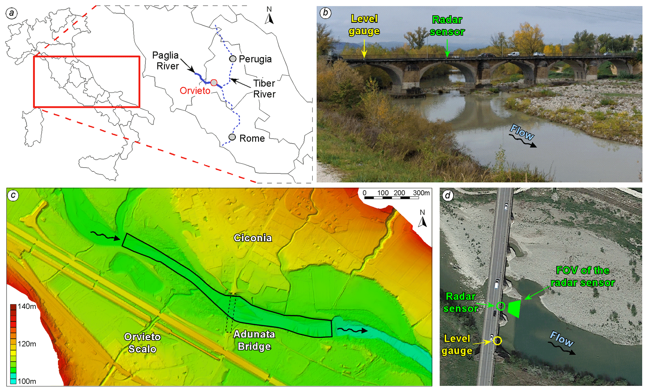
Figure 1(a) Location of the field site; (b) downstream view of the Adunata bridge on the Paglia River during normal flow condition (11 November 2021); (c) digital terrain model (DTM) nearby the Adunata bridge (dotted line), with the domain of the 3D CFD model (black line); and (d) location of the level gauge and of the radar sensor with the field of view (FOV) in an aerial image (© Google Earth, 2023).
The main thread of the flow is on the right-hand side of the river, and a large depositional area forms on the left-hand side just downstream of the bridge (Fig. 1b). The main channel axis is characterized by a significant curvature, bending to the left at the bridge section (Fig. 1c).
2.2 Available data
At the downstream side of the Adunata bridge, a water level gauge and a radar sensor for measuring the water surface velocity are located at the center of the first and second arch, respectively (Fig. 1d). The time resolution of both the sensors is 10 min. In addition, a number of flow rate measures and cross-sectional velocity distributions were provided by the Umbria Region Hydrological Service. The flow rate data were collected using a current meter by wading a few tens of meters downstream of the Adunata bridge in the period 2009–2011 (flow rate ranging between 3.3 and 14.3 m3 s−1), and from the bridge in the period 1995–2010 (flow rate ranging between 16.8 and 147 m3 s−1); additional flow rate data were collected using an acoustic Doppler current profiler (ADCP) some hundreds of meters upstream of the bridge in the period 2014–2019 (flow rate ranging between 0.37 and 45 m3 s−1). The official rating curve for the Adunata bridge, provided by ARPA Lazio, is based on these measurements.
As detailed in the following sections, the rating curve derived from current meter and ADCP data, the water levels, and the free-surface velocity data collected by the sensors mounted on the Adunata bridge were used to validate the hydrodynamic numerical models (Sect. 2.3 and Appendix A). The cross-sectional velocity distributions measured with the current meter just downstream of the bridge were used to further assess the spatial variability of the entropy-based velocity distributions, as detailed in Sect. 3.1.
2.3 Numerical model
The commercial CFD software STAR-CCM+ (Siemens) was used for the numerical simulations. It implements the finite-volume method to compute the flow field on unstructured, Cartesian computational grids. The software has been used and validated in several applications, including complex flows over deformed bathymetry, in the presence of obstacles (Chang et al., 2013; Kirkil et al., 2009; Lazzarin et al., 2023c, 2024b) and channel bends (Constantinescu et al., 2011, 2013; Koken et al., 2013). In the present application, the two-phase volume-of-fluid (VoF; Hirt and Nichols, 1981) method was used to track the water–air interface within the computational domain (Horna-Munoz and Constantinescu, 2018; Lazzarin et al., 2023b; Li and Zhang, 2022; Luo et al., 2018; Yoshimura and Fujita, 2020). STAR-CCM+ was used to solve the Reynolds-averaged Navier–Stokes (RANS) equations, in which the stress tensor in the momentum equations is related to the mean flow quantities by adopting the Boussinesq approximation. The eddy viscosity, μT, was determined by solving transport equations for the turbulent kinetic energy, k, and dissipation rate, ε, according to the realizable k–ε turbulence model (Shih et al., 1995), suitable for large-scale complex flows in natural rivers (e.g., Horna-Munoz and Constantinescu, 2018).
The computational domain reproduced a ∼1100 m long reach of the Paglia River (Fig. 1c), centered at the Adunata bridge. The average size of the grid elements was 1.0 m. Starting 100 m upstream of the bridge and up to 300 m downstream of the bridge, the grid was refined using elements with average length of 0.5 m. To capture the near-wall boundary layer well, a prism layer refinement with three layers was used to reduce the wall-normal thickness of the grid cells close to solid boundaries (i.e., the riverbed and bridge structure). The final computational grid was made of ∼4 million elements. A rough-wall, no-slip condition was imposed at the solid boundaries by means of a wall function (roughness height of 0.1 m at the bottom, and of 0.01 m at the bridge surfaces). The upper boundary of the computational grid was treated as a symmetry plane (i.e., slip condition) for the airflow. The water elevation at the outlet (i.e., downstream section) was kept fixed in time by imposing a suitable hydrostatic-pressure distribution. The value of the downstream level, for each of the simulated scenarios, was derived from an auxiliary two-dimensional (2D), depth-averaged hydrodynamic model calibrated on available data; the 2DEF model has been used for this purpose (see Appendix A for details on the model and its calibration/verification). A constant-in-time, logarithmic velocity distribution was imposed as the upstream boundary condition for the water fraction. For the air fraction (upper part of the numerical domain), zero velocity and zero pressure were imposed at the inlet and at the outlet, respectively. The simulations were advanced in time with an implicit, first-order discretization, until steady-state conditions were reached.
The 3D-CFD model was validated by comparing the surface velocity computed by the model with that measured by the radar sensor located downstream of the bridge (see the yellow bullets in Fig. A2c and d).
2.4 Flood events considered in the study
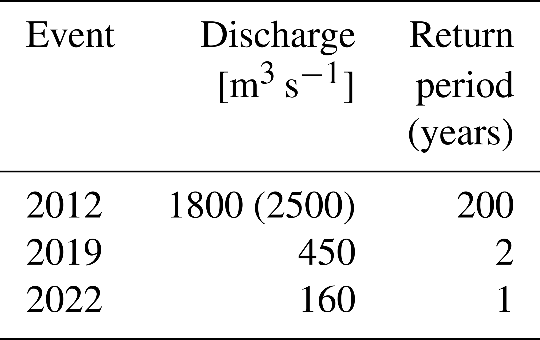
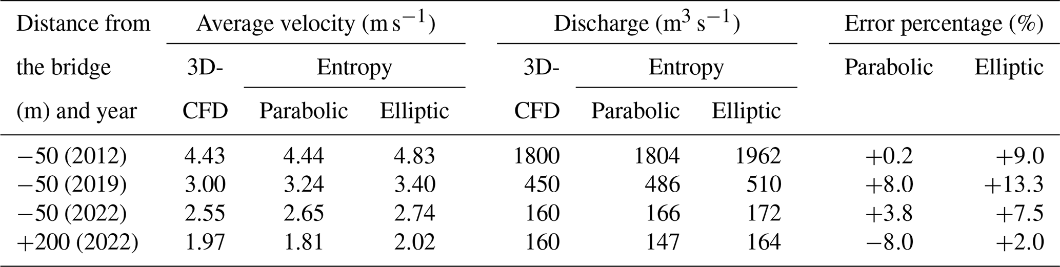
Three different steady flow conditions have been simulated with the 3D-CFD model STAR-CCM+, which correspond to the peak flow conditions of flood events that occurred in 2012, 2019, and 2022, as provided by the rating curve for the Adunata bridge (Table 1). In all three of the flow conditions, water flowed in the main channel and over the sediment bars that are dry in the low-flow condition of Fig. 1b and d. During the most severe flood of 2012, water also flowed on the floodplains adjacent to the main river and caused the incipient pressurization of flow below the bridge arches. The preliminary simulation carried out with the 2DEF depth-averaged model showed that, at the peak of the 2012 flood event, 700 m3 s−1 flowed through the floodplain, overflowing the bridge access roads, and 1800 m3 s−1 flowed within the main channel; this last value was used in the 3D-CFD simulation, which considered only the main channel of the river. The flood events of 2019 and 2022, although being quite ordinary, were the largest floods that occurred after the installation of the radar sensor for the surface velocity (thus, surface velocity data were not available for the 2012 flood).
Table 1Simulations performed in the present work. The value in brackets indicates the total discharge with consideration of the flow over floodplains, which is not considered in the 3D simulations.
2.5 Entropy theory
Entropy theory deals with physical systems that may have a large number of states from a probabilistic point of view. The concept of entropy is used for statistical inference, to determine a probability distribution function when the available information is limited to some average quantities, defined as constraints such as mean and variance. For the application of entropy to streamflow measurements, the pioneer was Chiu (1987), who developed a probabilistic formulation of the cross-sectional velocity distribution in open channels, in which the expected value of the point velocity is determined by applying the maximum entropy principle (Chiu, 1987, 1988, 1989). Using this probabilistic formulation, the velocity distribution is given analytically as a function of the cross-sectional geometry; of the dimensionless entropy parameter, M; and possibly of the depth at which the maximum velocity occurs (the so-called dip, h). There is a one-to-one correspondence between M and the ratio of mean to maximum velocity in the cross-section, which is defined as the entropic function, ϕ(M) (Chiu, 1991). In general, for a given river site, the magnitude of M and, in turn, of ϕ(M), mainly depends on hydraulic parameters such as roughness and hydraulic radius, whereas they are poorly affected by the flow discharge (Chiu and Murray, 1992; Moramarco and Singh, 2010). Moreover, ϕ(M) is consistently found to be nearly constant at different cross-sections through gauged river sites for different flow conditions (Moramarco and Singh, 2010; Ammari et al., 2022). This is because the value of ϕ(M) is associated with geometric and hydraulic characteristics that tend to vary smoothly within a river system (Ammari et al., 2022).
The estimation of cross-sectional velocity distribution, U(x,y), developed by Chiu (1989), was later simplified by Moramarco et al. (2004). Using this approach, one can divide the wet cross-sectional area into Nv verticals and determine the entropy-based velocity profile along each vertical as
where U is the time-averaged velocity, Umax(xi) is the maximum value of U along the ith vertical, xi is the distance of the ith sampled vertical from the left bank, h(xi) is the dip (i.e., the depth of Umax(xi) below the water surface), D(xi) the flow depth, and y is the vertical distance from the bed. The relationship between the entropic parameter, M, and the entropic function, ϕ(M), is (Chiu, 1989)
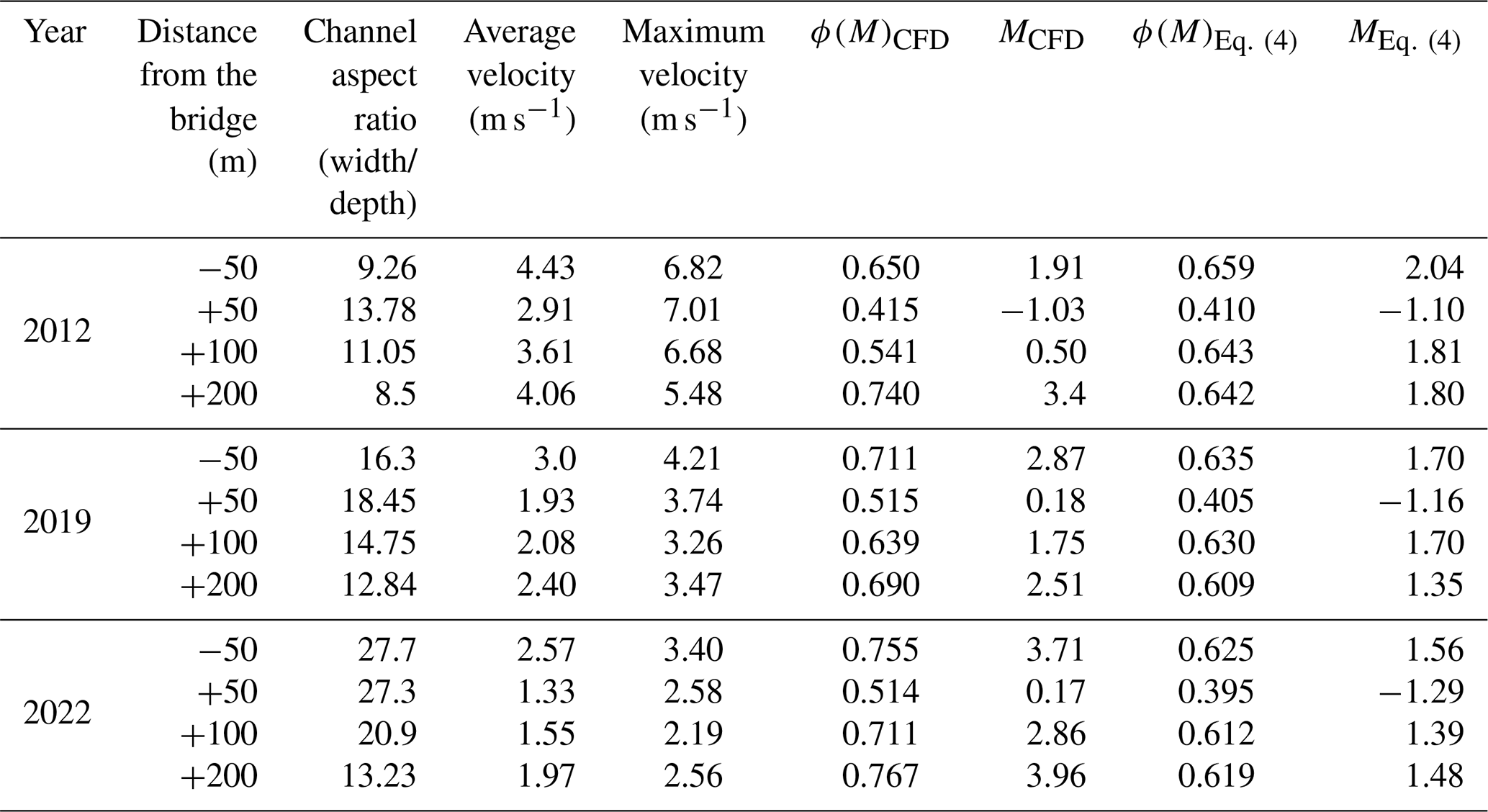
in which Um and UMAX are the average and maximum flow velocities within the entire cross-section. It is worth mentioning that Um represents the expected value of velocity that can be different from the observed mean velocity (Marini and Fontana, 2020). These two values are quite similar in the case of wide rivers (aspect ratio larger than 5). In the present research, considering the large aspect ratio for all cross-sections (Table 2), this hypothesis is valid.
Table 2Flow data for the cross-sections of Fig. 2 and the three considered flood events of Table 1. The values of the entropic function, ϕ(M), and parameter, M, are obtained from the 3D-CFD velocity distributions and estimated according to Eq. (4).
Introducing the variable , the velocity dip, h(xi), is estimated according to Yang et al. (2004) from the spanwise distribution of δ(xi), which is given as
in which xmin is the spanwise distance of the xi vertical from the nearest bank. Note that h(xi)=0 and δ(xi)=1 when the maximum velocity occurs at the free surface.
In the case of gauged cross-sections, ϕ(M) can be inferred from measured mean and maximum flow velocities (e.g., with ADCP). For ungauged sites, ϕ(M) can be estimated as (Moramarco and Singh, 2010)
where y0 is the vertical coordinate, taken from the bottom, where the velocity is zero; k is the von Karman constant; R is the hydraulic radius; n is the Manning roughness; D is the maximum water depth; and h is computed with Eq. (3) at the thalweg, i.e., where the water depth is maximum. According to van Rijn (1982), y0=0.065ξd90, where d90 is the 90th percentile for grain size and ξ a parameter ranging from 1 to 10 (Ferro, 2003; Moramarco and Singh, 2010).
When only the surface velocities, Usurf(xi), are available at a river site, then Umax(xi) can be estimated as (Fulton and Ostrowski, 2008)
For the current research, the methodological steps to estimate the cross-sectional velocity distribution (and hence the flow discharge) using entropy theory are as follows. The input data are the river-wide velocity distribution at the free-surface, Usurf, provided by the 3D-CFD model. When only the maximum value of Usurf is used as input, corresponding to the hypothetical case in which only point-sensor data are available, the spanwise distribution of Usurf is obtained by applying either a parabolic or an elliptical spanwise distribution (Bahmanpouri et al., 2022a). The velocity dip is computed using Eq. (3). The cross-sectional velocity distribution is then obtained using an iterative procedure, in which p denotes the iteration. At the first iteration, the entropic function, ϕ(M)p=1, is computed with Eq. (4), and Mp=1 is computed with Eq. (2). After computing the maximum velocity for each vertical, Umax(xi)p=1, with Eq. (5), Eq. (1) allows the entropic velocity distribution in the whole cross-section, , to be estimated. The following iteration starts by computing the average and the maximum flow velocities, Um and UMAX, from the velocity distribution obtained in the previous iteration and then , Mp using Eq. (2), Umax(xi)p with Eq. (5), and the velocity distribution U(xi,y)p with Eq. (1). The iterative procedure continues until the difference ϕ(M)p-ϕ(M)p−1 becomes lower than 0.01. For more details, the reader is referred to Moramarco et al. (2017).
The comparison between the entropy-based and the CFD-derived velocity distributions was performed considering four cross-sections (Fig. 2), at a distance of 50 m upstream and 50, 100, and 200 m downstream of the bridge, and the three flood events of 2012, 2019, and 2022 (see Table 1). The sections just upstream and downstream of the bridge are located at a distance of about 0.45 B from the bridge, with B∼110 m the width of the river at the bridge section. This is a short distance, relevant for the application given that the remote sensors for surface velocity (such as radar and large-scale particle image velocimetry (PIV)) have their field of view located some tens of meter upstream or downstream of the bridge. The sections far downstream are considered to assess how far the flow field is affected by the presence of the bridge.
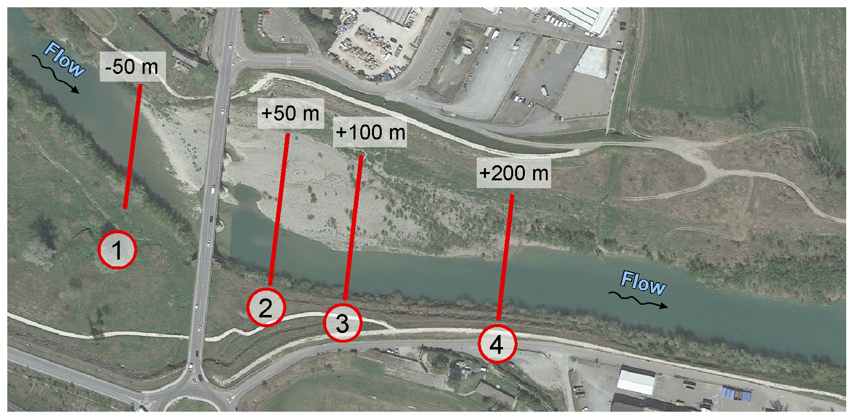
Figure 2Location of the Adunata bridge and of the four selected cross-sections (aerial image from © Google Earth 2023).
First, the study analyzed the variability of the entropy function, ϕ(M), at the four cross-sections, as derived from the cross-sectional velocity distributions provided by both the 3D-CFD model and the current meter measures (Sect. 3.1). Then, in applying the entropy model to estimate the cross-sectional velocity, two different procedures were considered. In the first one, the entropy model was forced with the river-wide distribution of the surface velocities computed by the 3D-CFD model (this is described in the following Sect. 3.2); in the second one, only the maximum value of the surface velocity computed by the 3D-CFD model was considered to be input for the entropy model (Sect. 3.3). The first procedure was applied to all the four cross-sections, whereas the latter was only applied to cross-sections 1 and 4, i.e., where the effects of the bridge piers are minimal and thus the spanwise velocity distribution is unimodal.
3.1 Variability of the entropy function
Some relevant parameters that characterize the flow field (e.g., aspect ratio, average and maximum velocity) at the selected cross-sections are presented in Table 2 for the peak flow condition of the three flood events. The values of the entropic function, ϕ(M)CFD, were first computed as the ratio of average to maximum velocity within the cross-section provided by the 3D-CFD model. Then, assuming the site as being ungauged, ϕ(M)Eq. (4) was estimated using Eq. (4) with d90=0.01 m (Pilbala et al., 2024) and a Manning parameter, n, equal to 0.035 ms at the upstream (−50 m) and far downstream sections (+100 and +200 m) and equal to 0.055 ms just downstream of the bridge (+50 m cross-section), where larger energy losses are expected because of the wakes generated by the bridge piers. The values of ϕ(M)Eq. (4), reported in Table 2 and corresponding with the points marked with dashed lines in Fig. 3b, were obtained using ξ=5 to compute y0 (Sect. 2.5 just after Eq. 4), and the gray band was obtained by varying ξ in the range [1, 10]. Finally, the values of the entropic parameter associated with the different values of ϕ(M) are computed using Eq. (2).
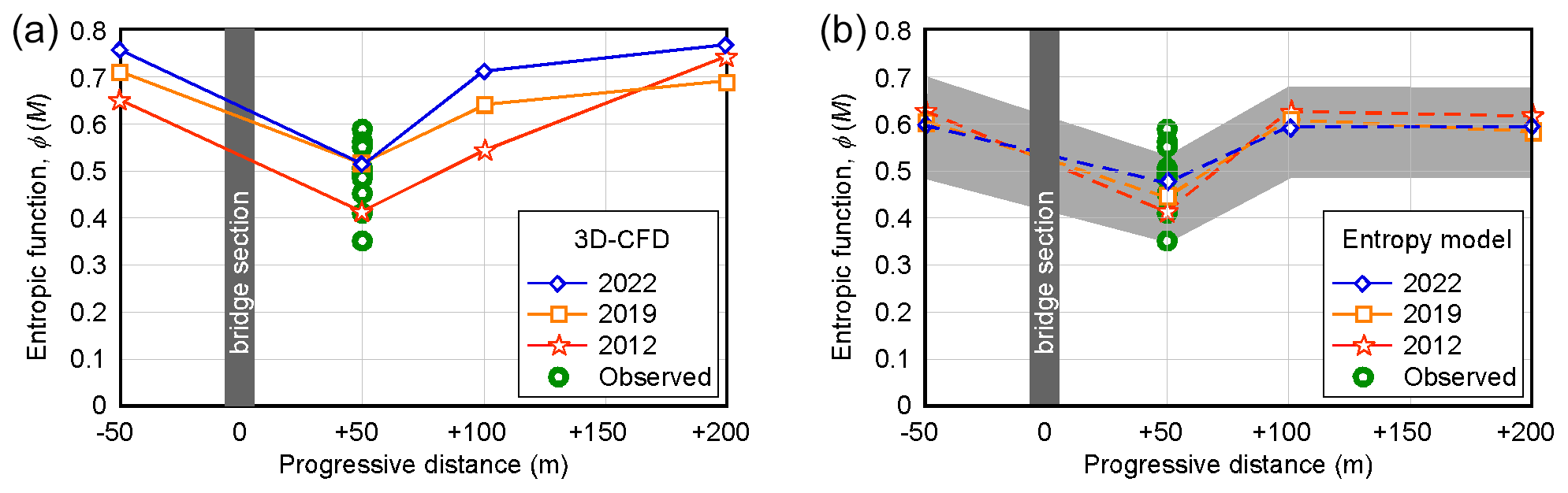
Figure 3Entropic function ϕ(M), for the different simulated scenarios, as a function of the distance from the bridge (positive downstream), (a) computed from the 3D-CFD flow fields and (b) estimated with Eq. (4), where the lines refer to the average values, and the gray band is obtained by varying the reference height y0 in Eq. (4) within the expected range. Green circles refer to data derived from velocity distributions measured with the current meter just downstream of the bridge.
Since the entropic function is typically assumed to be constant for all flow conditions at a given cross-section, it is of interest to analyze its actual variation by exploiting the flow fields provided by the 3D-CFD model and to see the effectiveness of their first-guess estimates obtained using Eq. (4). The values of ϕ(M) reported in Table 2 are plotted in Fig. 3 as a function of the downstream distance from the bridge. At the first cross-section downstream of the bridge (i.e., cross-section 2), although referring to different flow conditions, the values of the entropic function computed with the 3D-CFD and the current meter velocity distributions show the same magnitude, further confirming the reliability of the 3D-CFD model. The first-guess estimates of ϕ(M) in Fig. 3b, although they have a marginal role on the entropy-based computations, show a similar trend to the 3D-CFD estimates (Fig. 3b), provided that the increased Manning parameter is used at the section just downstream of the bridge. The need to calibrate such an increased Manning parameter complicates efforts in the case of disturbed flows.
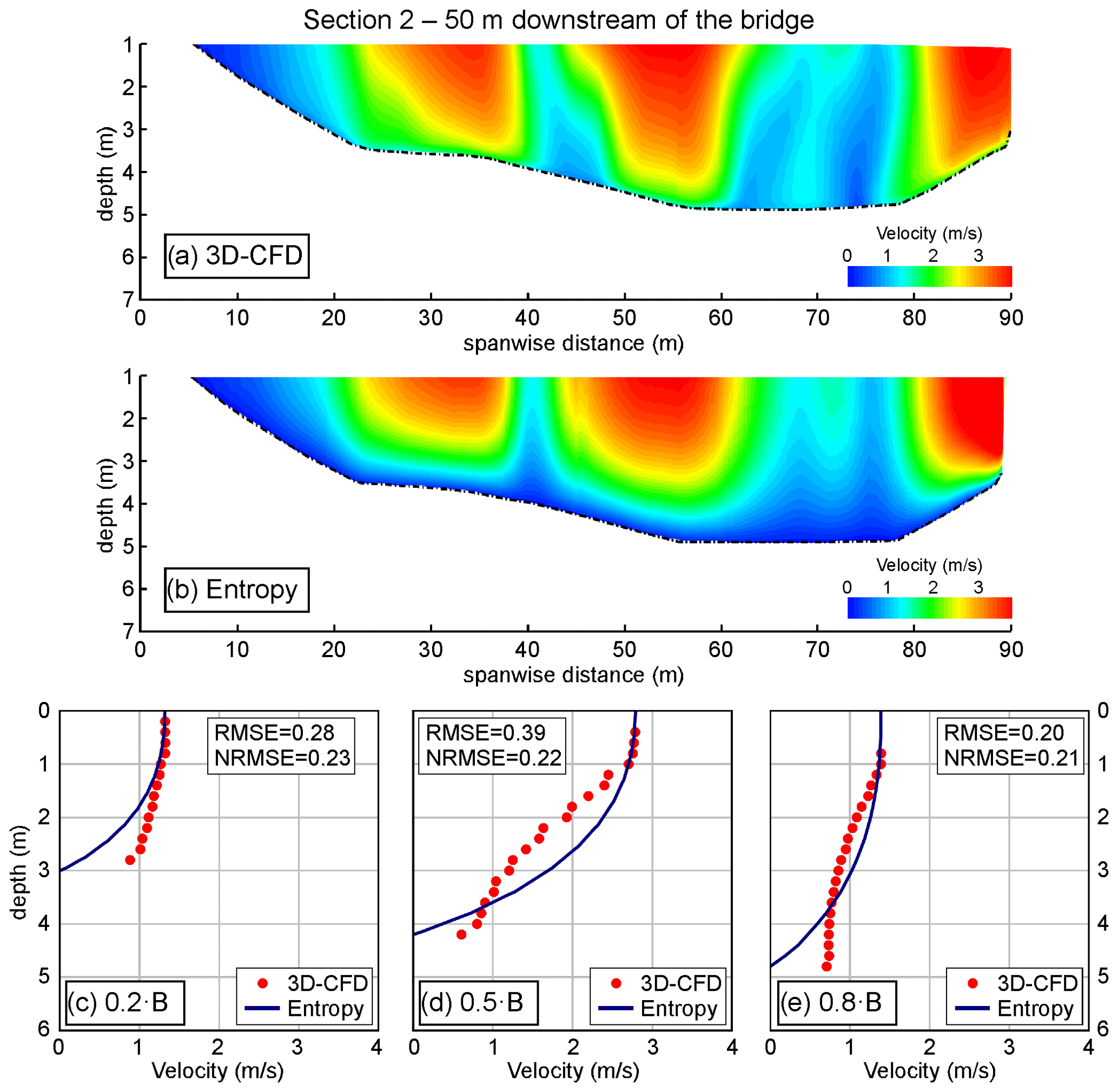
Figure 4Flood event of 2019, cross-section 2 (50 m downstream of the bridge). Velocity distributions provided by (a) the 3D-CFD model and (b) the entropy model forced with the river-wide distribution of the free-surface velocity. Comparison of vertical distributions of velocity at 0.2 B (c), 0.5 B (d), and 0.8 B (e), where B is the width of the cross-section.
For each flood event, at cross-sections 1 and 4, i.e., where the flow field is not characterized by the wakes generated by the bridge piers, the entropic function assumes similar values, which can be identified as “undisturbed” values. The variability of such undisturbed values of ϕ(M) with the flow rate is relatively small, as all the values fall in the range , in agreement with the range found by Bahmanpouri et al. (2022b) for similar European rivers. By contrast, at cross-sections 2 and 3, just downstream of the bridge, the values of ϕ(M) are consistently reduced due to the effect of the bridge. In the largest flood event of 2012, which produced near-pressure flow conditions at the bridge with marked localized increasing of the flow velocity, ϕ(M)CFD equals 0.415 at cross-section 2, corresponding to . The low value of ϕ(M) and the negative value of M attest the markedly non-uniform distribution of the velocity (i.e., the maximum velocity in this cross-section is much higher than the average velocity). A sensible reduction is still present 100 m downstream of the bridge (cross-section 3). For the moderate peak flows of 2019 and 2022 events, the entropic function recovers undisturbed values already at cross-section 3, i.e., 100 m downstream of the bridge.
This first analysis suggests that assuming constant values of ϕ(M) can be reasonable in undisturbed river reaches; however, in the case of irregular flow fields induced by the interaction with in-stream structures, the entropic function ϕ(M) can vary with respect to undisturbed values, and, in addition, it can show significant variations with the flow rate.
Table 3Comparison between 3D-CFD outputs and entropy-based estimations forced with the river-wide distribution of the free-surface velocity.
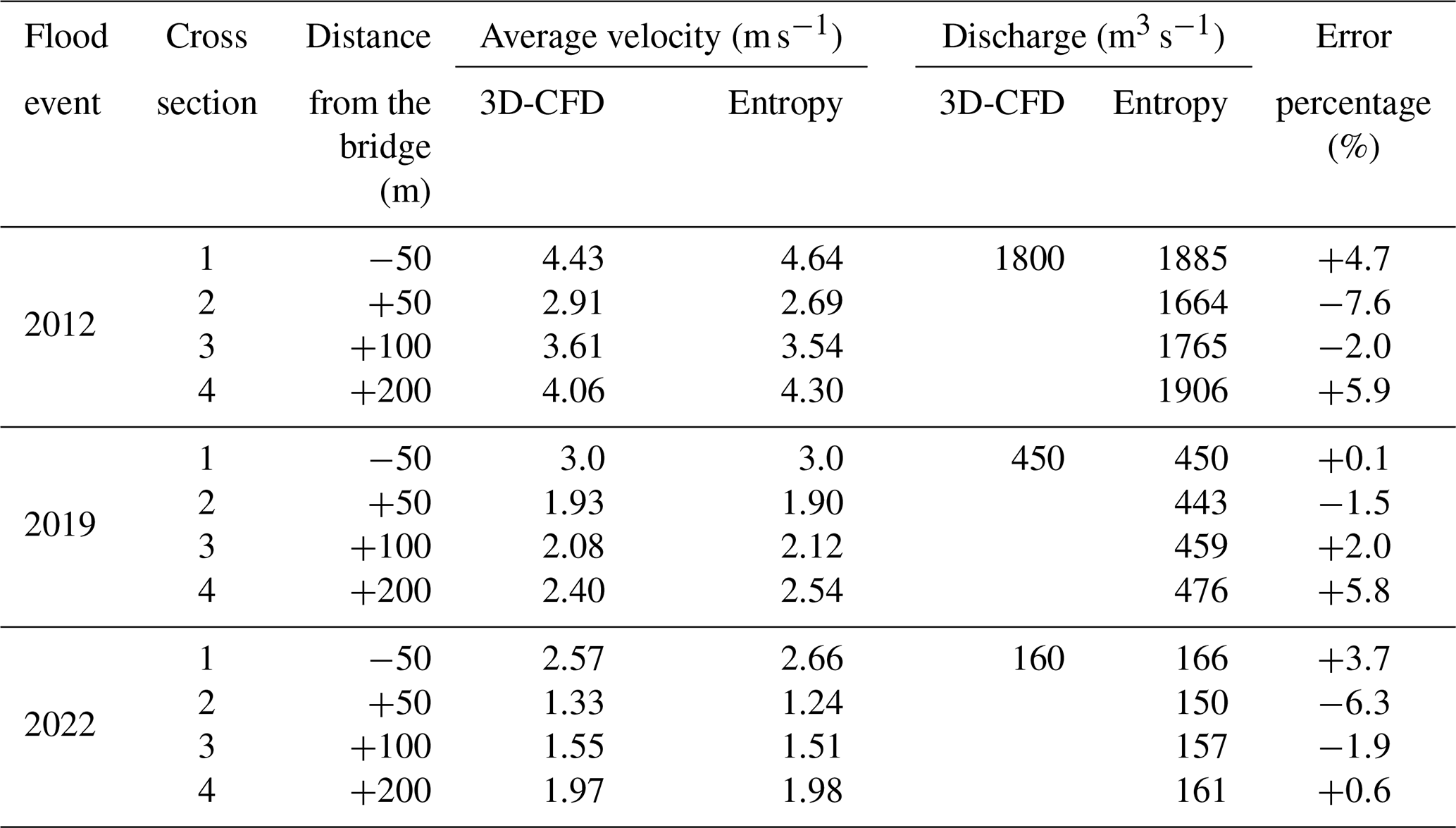
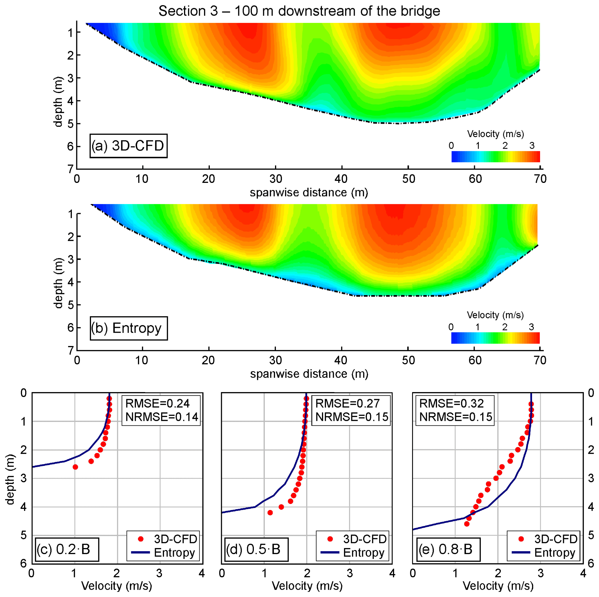
Figure 5Flood event of 2019, cross-section 3 (100 m downstream of the bridge). Velocity distributions provided by (a) the 3D-CFD model and (b) the entropy model forced with the river-wide distribution of the free-surface velocity. Comparison of vertical distributions of velocity at 0.2 B (c), 0.5 B (d), and 0.8 B (e), where B is the width of the cross-section.
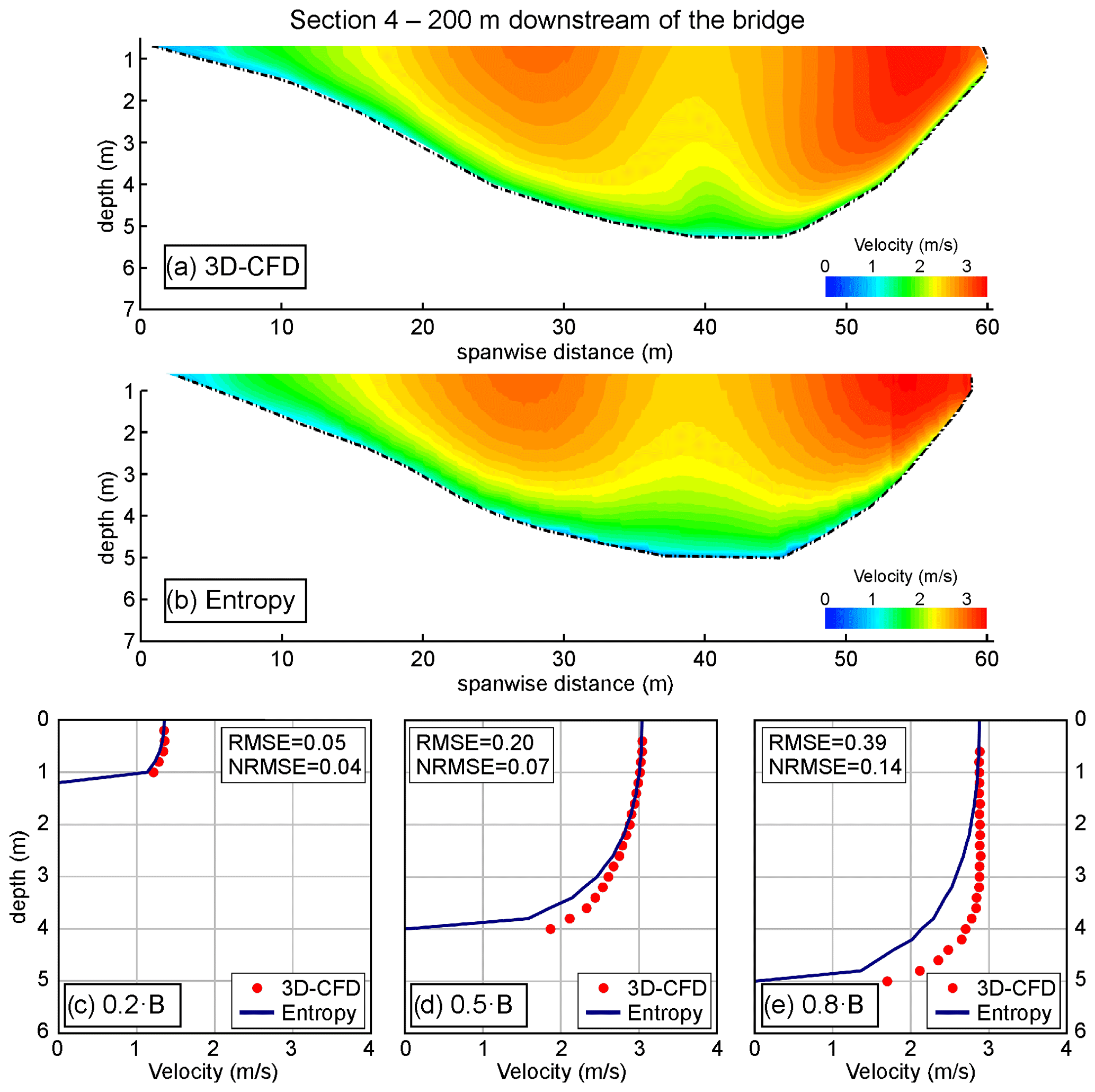
Figure 6Flood event of 2019, cross-section 4 (200 m downstream of the bridge). Velocity distributions provided by (a) the 3D-CFD model and (b) the entropy model forced with the river-wide distribution of the free-surface velocity. Comparison of vertical distributions of velocity at 0.2 B (c), 0.5 B (d), and 0.8 B (e), where B is the width of the cross-section.
3.2 Entropy model forced with the river-wide profile of free-surface velocity
The efficacy of the entropy model is tested here for the case in which the surface velocity is known for all the width of the cross-section. This could be the case in which the river-wide surface velocity is estimated from imaging techniques (e.g., Eltner et al., 2020; Schweitzer and Cowen, 2021). The results, in terms of cross-sectional velocity distributions, are presented for brevity only for the intermediate peak flow of the 2019 flood event and for the most challenging cross-sections just downstream of the bridge, where the flow field is disturbed by the pier wakes. The same results, for the peak flows of 2012 and 2022 events, are provided in the Supplement.
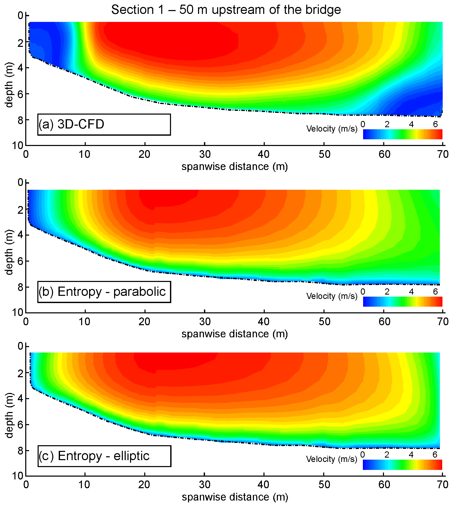
Figure 7Flood event of 2012, cross-section 1 (50 m upstream of the bridge). Cross-sectional velocity distribution computed with the 3D-CFD model (a). Entropy theory with parabolic spanwise velocity distribution (b) and entropy theory with elliptic spanwise velocity distribution (c).
Figure 4 presents the cross-sectional velocity distribution 50 m downstream of the bridge (cross-section 2). As shown by the 3D-CFD flow field (Fig. 4a) and reflected in the low value of ϕ(M) for this cross-section (Table 2 and Fig. 3), the effect of the piers is very strong, such that there is a clearly uneven distribution of the cross-sectional velocity because of the wakes developing downstream of the piers. Just downstream of the bridge, due to the presence of the bridge arches, the flow field provided by the 3D-CFD model is configured as a sort of partial orifice flow that increases the vertical uniformity of the velocity distribution compared to a uniform shear flow. Of course, the entropy model cannot capture such localized flow features, which entails some difference in the patchiness of the physics-based and the entropy velocity distributions (Fig. 4a–e). Despite that, using the river-wide distribution of the surface velocity provided by the CFD simulation as input, the entropy model can reliably capture the salient features of the cross-sectional velocity distribution. Figure 4c–e highlight the comparison of 3D-CFD and entropy flow velocities along three verticals located at 0.2, 0.5, and 0.8 B (where B is the channel width). Compared to the results of the 3D-CFD model, the entropy approach underestimates the velocity close to the bed. Since the velocities and the volumetric fluxes are still relatively small near the bed, these discrepancies marginally affect the estimation of the section-averaged velocity and, consequently, of the total discharge (Table 3). The percentage error is larger (7.6 %) for the very high-flow condition of the 2012 event (see Supplement), due to the accentuation of orifice-flow conditions associated with the higher water levels.
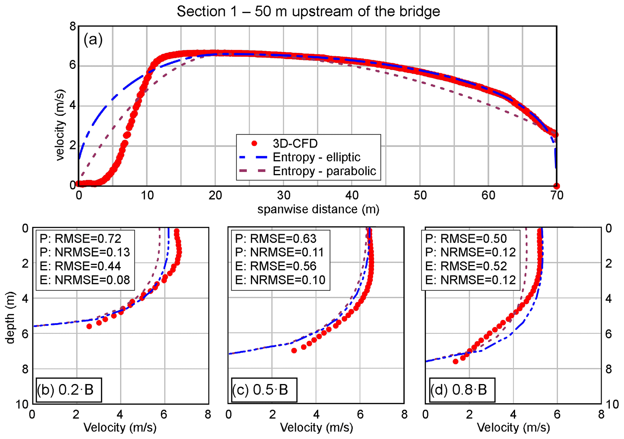
Figure 8Flood event of 2012, cross-section 1 (50 m upstream of the bridge). Spanwise distribution of the surface velocity (a) and comparison of vertical distributions of velocity at 0.2 B (b), 0.5 B (c), and 0.8 B (d).
Figure 5 depicts the cross-sectional velocity distributions at a larger distance from the bridge, i.e., at cross-section 3, placed 100 m downstream of the bridge. The visual comparison with Fig. 4 suggests that the effects of the piers on the flow field are reduced because of the increased distance, and the cross-sectional distribution provided by the 3D-CFD model (Fig. 5a) appears to be more regular. The statistical analysis confirms that in this case the entropy model (Fig. 5b) is able to simulate the velocity profiles with a higher accuracy.
Figure 6 shows the cross-sectional velocity distributions of 3D-CFD and entropy models for cross-section 4, located 200 m downstream of the bridge. Compared to cross-section 3, the effect of the bridge piers is further reduced because of both the distance and the more compact shape of the cross-section. Since the effect of the bridge piers is minimum, the statistical analysis shows a better agreement of the entropy model results with the CFD-based data. Though areas with relatively high velocities are still visible in simulations with higher values of the discharge (i.e., events of 2012 and 2019), for the high-flow conditions of 2022, the effect of the bridge pier has completely vanished. Therefore, the lower the flow discharge, the lower the distance from the bridge to recover undisturbed flow conditions.
The results presented here show that, when the river-wide distribution of the free-surface velocity is provided, the entropy method provides good estimations of the cross-sectional velocity distribution even when the influence of bridge piers, and thus the unevenness of the flow field, is relevant. The main discrepancies are observed in low-velocity regions, which slightly affect the estimation of the flow discharge. Table 3 lists some statistics and error percentages for the depth-averaged velocity and discharge estimations for all cross-sections and the three events considered. The estimations provided by the entropy method are in good agreement with results of CFD model, both upstream and downstream of the Adunata bridge. Though the accuracy is slightly reduced downstream of the bridge, the results are also reliable in the vicinity of the structure (i.e., at cross-section 2), suggesting the applicability of the entropy model to estimate the flow discharges, even in the case of irregular distributions of the cross-sectional velocity, provided that the river-wide distribution of the surface velocity is used as input data.
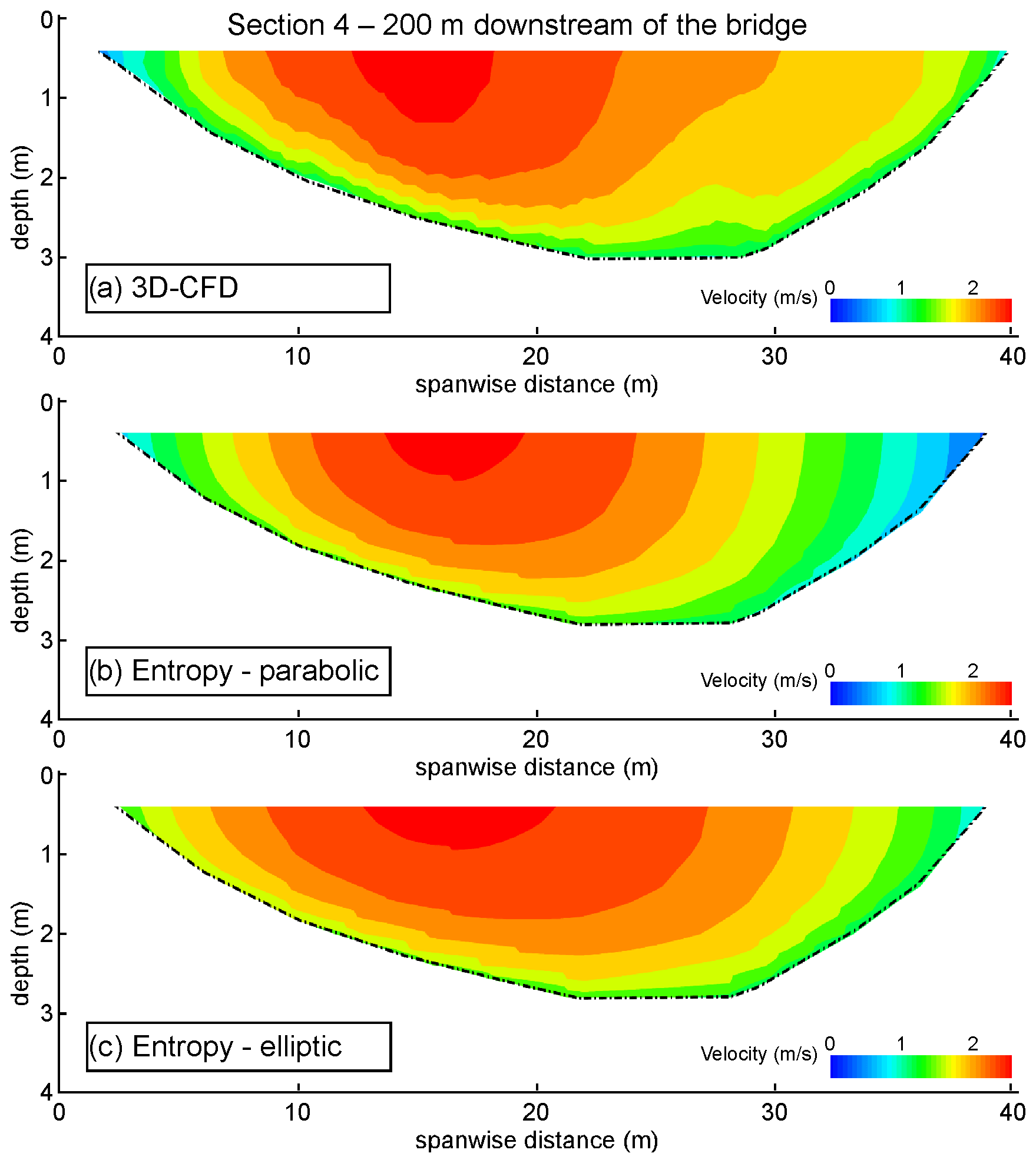
Figure 9Flood event of 2022, cross-section 4 (200 m downstream of the bridge). Cross-sectional velocity distribution computed with the 3D-CFD model (a). Entropy theory with parabolic spanwise velocity distribution and (b) entropy theory with elliptic spanwise velocity distribution (c).
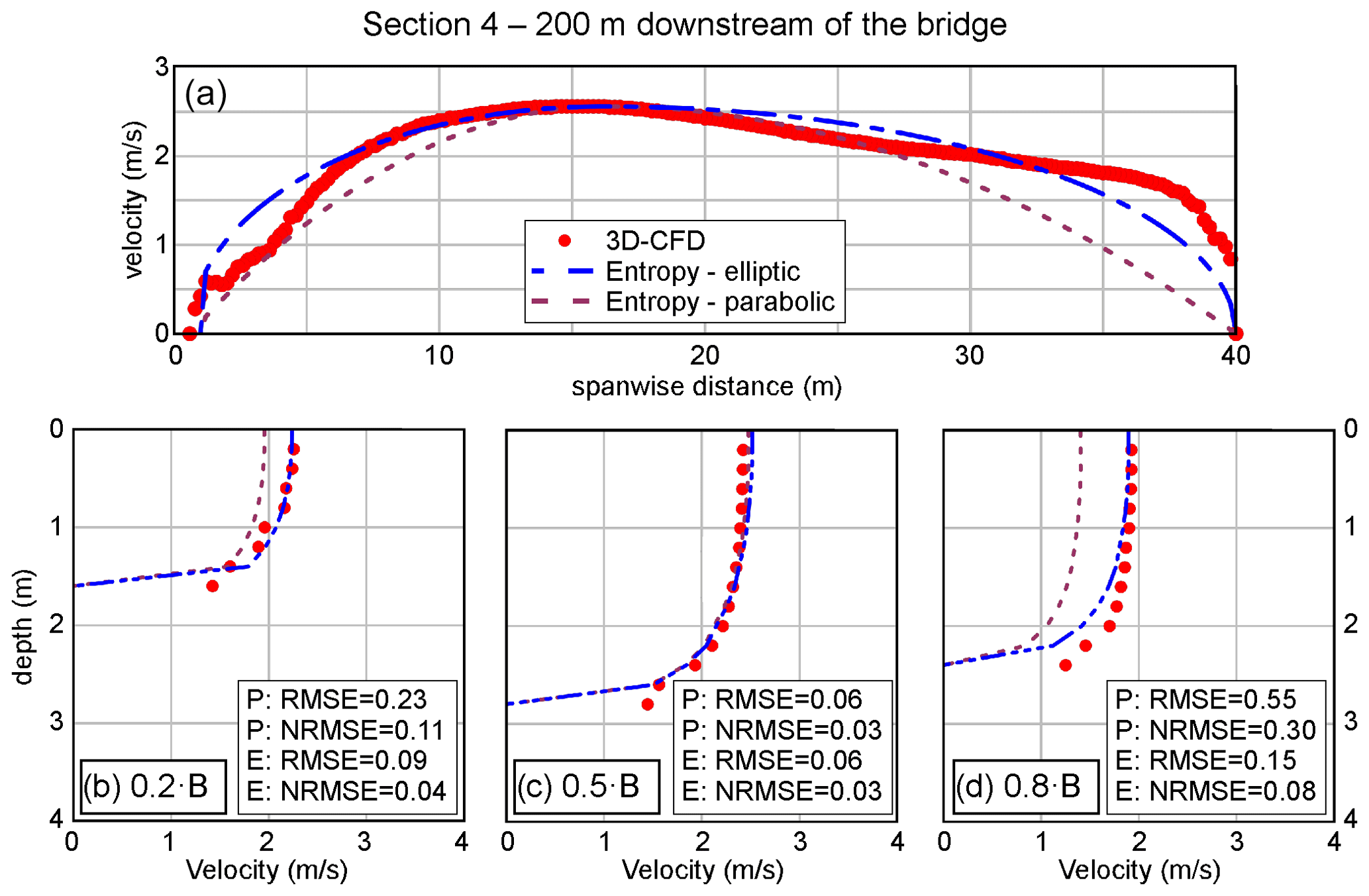
Figure 10Flood event of 2022, cross-section 4 (200 m downstream of the bridge). Spanwise distribution of the surface velocity (a) and comparison of vertical distributions of velocity at 0.2 B (b), 0.5 B (c), and 0.8 B (d).
3.3 Entropy model forced with a single value of free-surface velocity
In this section, the results are presented considering only a single value of the surface velocity as input for the entropy model, which corresponds to the maximum surface velocity predicted by the 3D-CFD model. Two different spanwise velocity distributions are enforced in the entropic model, namely a parabolic spanwise distribution (PSD) and an elliptic spanwise distribution (ESD). Of course, applying the entropy model using a unique value of the velocity is particularly sensitive to this value and supposes a unimodal velocity distribution in the spanwise direction. For this reason, this kind of approach cannot be used in the cross-sections immediately downstream of the bridge, where the spanwise velocity distribution is markedly irregular (see e.g., Fig. 4). Herein, the results are presented for cross-section 1, located 50 m upstream of the bridge for the high-flow condition of the 2012 event, and for cross-section 4, located 200 m downstream of the bridge, for the modest peak flow condition of the 2022 event, where the effect of bridge piers on the velocity distribution wears off in a shorter distance.
Figure 7 shows the distribution of the surface velocity based on the 3D-CFD outputs and both the PSD and ESD entropy models. The agreement of both the PSD and the ESD is generally good in the central and the right parts of the channel and less good in the left part of the channel. Here, due to the irregular bathymetry (i.e., gravel deposit), the 3D-CFD model predicts localized stagnation zones that cannot be captured by the entropy model based on a single value of the surface velocity. This is confirmed by Fig. 8, which shows the cross-sectional distribution of the surface velocity and three vertical profiles. In the perspective of estimating the flow discharge, the lateral discrepancies represent a minor limit, as the central part of the cross-sections conveys the largest part of the total discharge.
Table 4Comparison between 3D-CFD and entropy-based outputs considering a single surface velocity.
Overall, the cross-sectional velocity distributions based on ESD seem more accurate than those based on the PSD: they provide similar results at the center of the channel, but the parabolic distribution generally underestimates the flow velocity close to the banks. Both cross-sectional and vertical distributions of the velocity profiles (Figs. 7a and 8c) highlight the existence of a velocity dip; i.e., the maximum velocity is below the water surface, particularly at the center of the channel. This is generally the consequence of secondary currents superposed on the main flow (Termini and Moramarco, 2020). Yang et al. (2004) and Moramarco et al. (2017) reported that for large aspect ratios of channel flow, , the dip phenomenon appears primarily near the sidewall region, whereas for relatively low aspect ratios ( for cross-section 1) the velocity dip is generally located at the center of the channel (Bahmanpouri et al., 2022a, b; Kundu and Ghoshal, 2018; Moramarco et al., 2017; Termini and Moramarco, 2020). In this case, the 3D flow field from the CFD simulation shows that the dip depends on the counter-clockwise rotating secondary current generated by the upstream right-handed bend. Indeed, rotational inertia makes these curvature-induced helical flow structures propagate downstream for relatively long distances (Dominguez Ruben et al., 2021; Lazzarin and Viero, 2023; Thorne et al., 1985).
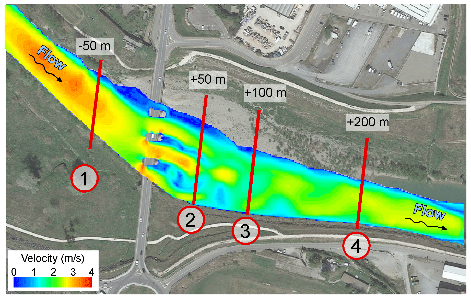
Figure 11Flood event of 2022. Color map of the instantaneous surface velocities computed with the 3D-CFD model for the Paglia River at the Adunata bridge (aerial image from © Google Earth, 2023).
The velocity distribution at cross-section 4 (200 m downstream of the bridge) is presented in Fig. 9 for the moderate peak flow condition of the 2022 event. For this cross-section, in the 3D-CFD results (Fig. 9a), the maximum surface velocity is located on the left side of the channel, rather than at its center (this aspect is discussed in the following). Forced with the maximum water surface velocity, the entropy model reproduces the velocity field in the central part of the riverbed well. Larger discrepancies are instead observed in the lateral part of the cross-section, with the elliptic spanwise distribution (ESD) that performs slightly better than the parabolic (PSD), particularly in the right side. Figure 10 shows the cross-sectional distribution of the surface velocity and the velocity distribution along three verticals. In terms of cross-sectional average velocity and flow discharge, both the PSD and ESD produce error that are lower than 10 % (Table 4), larger than those obtained using the river-wide surface velocity as input for the entropy model.
A last point worth discussing regards the unusual cross-sectional distribution of flow velocity in Sect. 4 (Fig. 9a). The reason that the 3D-CFD model locates the maximum velocity on the left of the thalweg is the alternate vortex shedding occurring downstream of the bridge piers, which propagates beyond the last considered cross-section. This is evident in the map of instantaneous surface velocity of Fig. 11. This particular occurrence poses interesting questions on the application of the entropy model to estimate the flow discharge downstream of in-stream structures. First, the spanwise location of the maximum surface velocity is subject to a periodical shift, which prevents its correct detection by means of a fixed sensor with a small-size field of view, like the one mounted on the Adunata bridge. Secondly, marked time-varying flow fields, which occasionally (or periodically) deviate from nearly uniform flow conditions, can hardly be captured by any preset velocity distribution. To alleviate the problem, the periodic signal of surface velocity can be filtered, which is equivalent to looking at time-averaged modeled flow fields; this requires knowing the frequency of vortex shedding.
The results shown in this section confirm the general accuracy of the entropy model in predicting the cross-sectional velocity distributions. As expected, when using a single value of velocity in place of the river-wide distribution of surface velocity, the accuracy of the method slightly decreases. Provided that using a single velocity is beyond the scope of the method when the spanwise velocity distribution is markedly irregular, the entropy approach can still be forced with a single surface velocity and produce accurate results, when there is no evidence of strong disturbances of the flow. Indeed, such an approach cannot capture marked unevenness in the flow field, as shown in the case of the lateral low-velocity regions at cross-section 1 for the 2012 event (Fig. 7) and in the time-varying flow field of cross-section 4 for the 2022 event (Fig. 9).
The present study investigated the ability of the entropy-based method to estimate the cross-sectional distribution of velocity, as well as the associated river discharge, for different flow conditions in a representative case study. As sensors for continuous monitoring of water level and surface velocity are often mounted on bridges, we analyzed a stretch of the Paglia River where a multi-arch bridge with thick piers, hosting a level gauge and a radar sensor, strongly affects the flow field. A 3D-CFD model was set up to obtain reliable, physics-based velocity distributions at relevant cross-sections, both upstream and downstream of the bridge. The entropy model was then applied to reproduce this set of velocity distributions, using the bathymetric data and the CFD-computed surface velocity as input data.
As a first point, the study highlighted the potential of using accurate, physics-based 3D-CFD models to deepen the knowledge of rivers and, specifically, of theoretical methods for discharge estimation. Indeed, 3D-CFD models provide pictures of complex flow fields that are more complete than, e.g., ADCP measures, in terms of spatial and temporal distribution and, above all, valid for high-flow regimes, which typically prevent any direct measurement of the flow field beneath the free surface. This entails unexplored chances of outlining best practices in the use of simplified methods for continuous discharge monitoring and, as a consequence, to improve their accuracy.
According to the present analysis, the entropy model revealed remarkable skills in also reproducing disturbed and uneven flow fields when the river-wide distribution of the surface velocity is used as input data. This occurred also just downstream of the bridge, where the pier-induced wakes made the velocity distribution multimodal and extremely irregular, with error on discharge estimates lower than 8 %. The availability of innovative measuring techniques, able to collect river-wide surface velocity data at a relatively low cost, adds value to the present findings.
On the other side, the accuracy of the entropy model is reduced when only the maximum surface velocity is used as input data, so that the spanwise velocity distribution has to be assumed on a theoretical basis (e.g., parabolic or elliptical). While such a method is absolutely discouraged in the case of disturbed flow fields (e.g., downstream of in-stream structures), it still provides accurate estimates when the velocity field is sufficiently smooth.
As a final recommendation, measuring instruments and sensors for surface velocity become more effective when placed upstream of in-stream structures, i.e., where the flow field is only marginally affected by the structure and both the water surface elevation and the velocity distribution are far more regular.
A main limitation of the present methodological approach is that it relies in the assumption of a fixed bed in both the CFD analysis and the application of the entropic model. In natural rivers, bed scouring during severe flood events and the ensuing formation of local deposits, especially close to in-stream structures such as bridges, can alter the bathymetry and, in turn, the velocity distribution and the discharge estimates. In the case of a movable bed and in the absence of protection measures (e.g., riprap or bed sills), the uncertainty associated with the local bed mobility has to be evaluated with due care. Future research on more complex scenarios that still need a comprehensive assessment, and which could largely benefit from physics-based numerical modeling, will include the case of mobile beds and the analysis of stage-dependent variations of cross-sectional velocity distribution, particularly in the case of compound cross-sections that are typical of lowland natural rivers.
To impose the boundary conditions in the 3D-CFD model, a 2D depth-averaged model of a longer stretch of the Paglia River has been set up. We used the 2DEF finite-element model (Defina, 2003; Lazzarin et al., 2023a, 2024c; Viero, 2019; Viero et al., 2013, 2014), which solves a modified version of the shallow water equations (SWEs) that allow for a robust treatment of wetting and drying over irregular topographies (D'Alpaos and Defina, 2007; Defina, 2000). The SWEs are written as
in which hs is the free surface elevation; t is the time; ∇ and ∇⋅ denote the 2D gradient and divergence operators, respectively; is the depth-integrated velocity (i.e., the unit-width discharge); Y is the equivalent water depth (i.e., the volume of water per unit area); η(hs) is a storativity coefficient to account for the wetted fraction of the domain; is the bed shear stress, evaluated using the Gauckler–Strickler formula; ρ is the water density; and Re is the horizontal components of the Reynolds stresses, modeled according to the Boussinesq approximation. A mixed Eulerian–Lagrangian approach allows the total derivative of the flow velocity in the momentum equations to be evaluated using finite differences and a backward tracing technique based on the method of characteristics (Defina, 2003; Giraldo, 2003; Walters and Casulli, 1998). Then, the SWEs are solved with a finite-element method, based on triangular, unstructured grids. The model also allows 2D triangular elements to be coupled with 1D elements (either open or closed sections) to model the minor hydraulic network efficiently; other 1D elements are used to model particular devices, such as pumps and weirs (Martini et al., 2004). The model has been successfully used to simulate flows in various rivers (e.g., Mel et al., 2020a, b; Viero et al., 2019; Baldasso et al., 2023); its effectiveness have also been demonstrated in different research fields, such as lagoon and marine environments (e.g., Carniello et al., 2012; Pivato et al., 2020; Tognin et al., 2022; Viero and Defina, 2016).
In the present case, the computational mesh covered a stretch of the Paglia River about 7 km long, from 600 m upstream of the Adunata bridge to the confluence with the Tiber River, including floodable floodplains (Fig. A1). The average mesh size ranged from 10 m in the riverbed near the Adunata bridge to 30 m in the floodplains and far downstream of the Adunata bridge. The computational mesh included 61 000 triangular elements, 16 1D elements to simulate underpasses, and 4 1D weir elements to simulate the sill located 500 m downstream of the Adunata bridge.
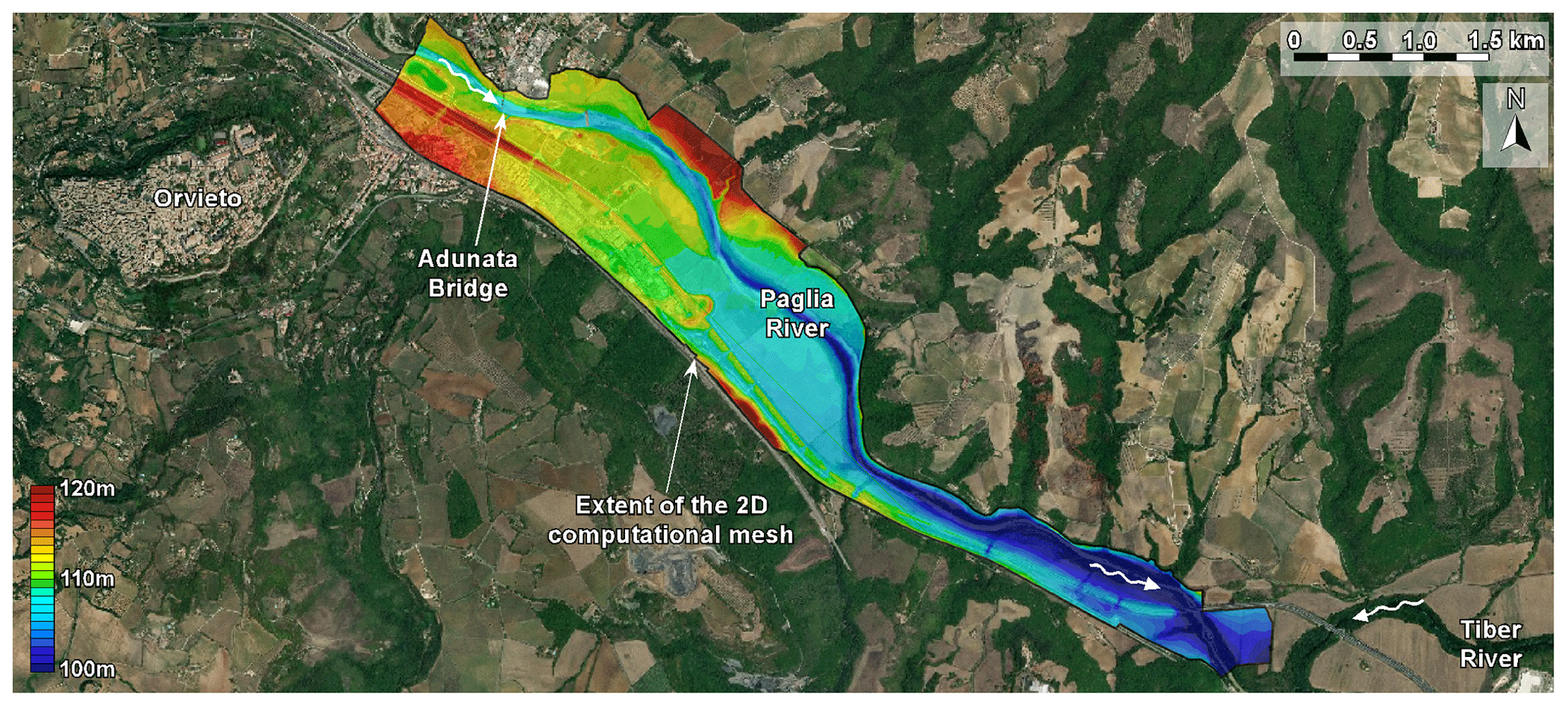
Figure A1Spatial extent of the 2D computational mesh (aerial image from World Imagery). The color map shows the bottom elevation of the grid elements derived from the lidar-based DTM.
The inflow hydrographs, prescribed at the upstream mesh inlet, were derived from water levels measured at the Adunata bridge using the associated rating curve. At the outlet, an arbitrary rating curve was applied as the downstream boundary condition; a sensitivity analysis showed that, because of the distance from the Adunata bridge, this boundary condition did not produce any perceivable effect in the water levels simulated at the study site.
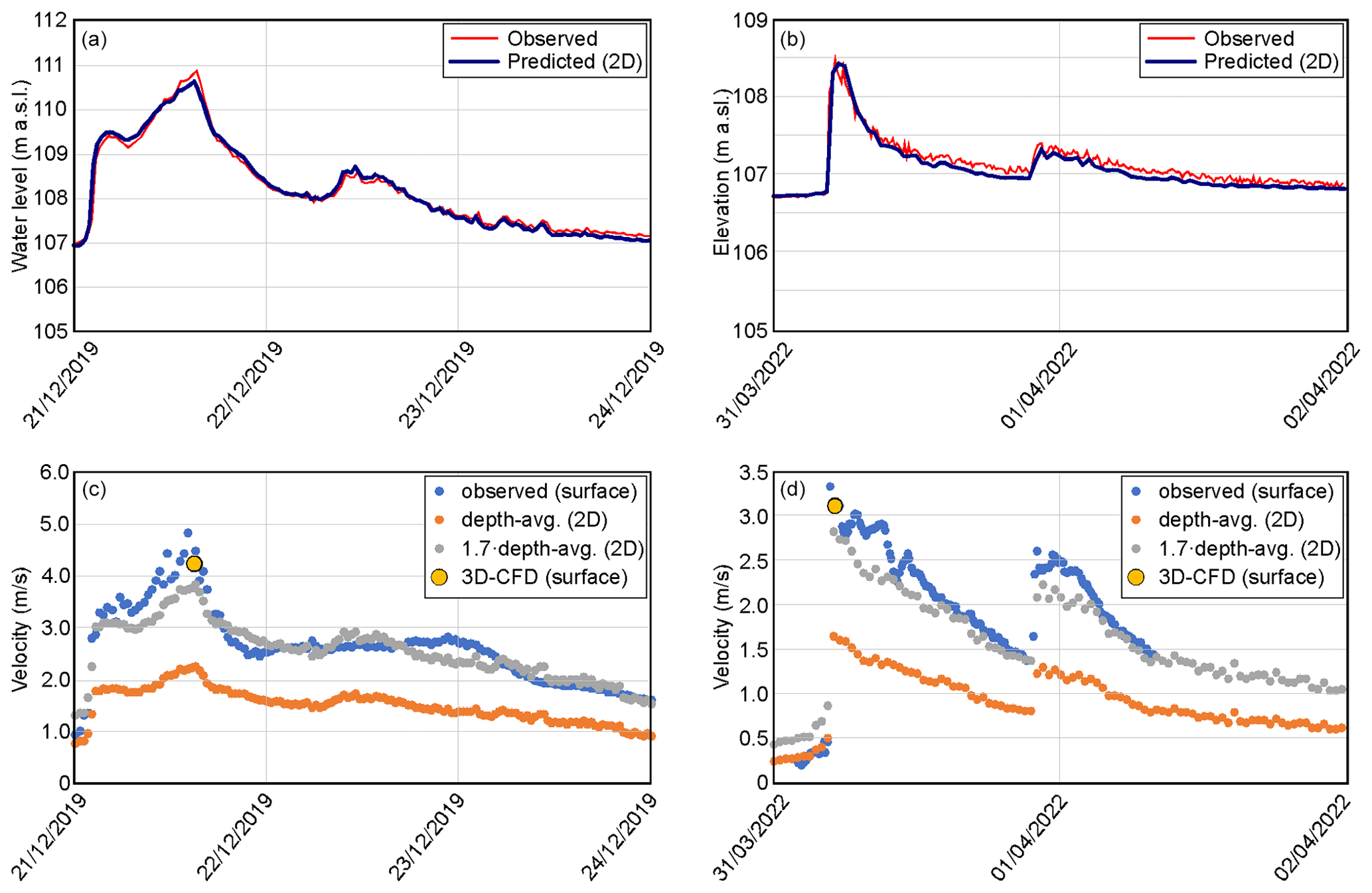
Figure A2Observed (red) and predicted (blue) water levels at the Adunata bridge gauging station for the flood events of 2019 (a) and 2022 (b). Observed and predicted water velocity for the flood events of 2019 (c) and 2022 (d).
Different Gauckler–Strickler coefficients were assigned to the different parts of the domain (e.g., floodplains and densely vegetated areas) based on the soil cover. The value assigned to the main riverbed were calibrated to match the time series of the water levels measured at the Adunata bridge gauging station for the 2019 flood event (Fig. A2a), and, for the most severe flood event that occurred in 2012, the model results were also checked in terms of extent of flooded areas. The minor flood of 2022 was used to verify the model (Fig. A2b). Finally, the depth-averaged velocity just downstream of the Adunata bridge was compared with the free-surface velocity measured by the radar sensor. Due to the use of a coarse grid and to the depth-average assumption, the 2D model underpredicted the measured water surface systematically (Fig. A2c and d); however, using an amplification factor of 1.7 (gray dots in Fig. A2c and d), the predicted values were quite similar to the measured ones.
Data are available on request from the authors.
The supplement related to this article is available online at: https://doi.org/10.5194/hess-28-3717-2024-supplement.
Conceptualization: FB, TL, SB, TM, DPV. Formal analysis: FB and TL. Funding acquisition: TM. Investigation: FB and TL. Methodology: FB, TL, SB, TM, DPV. Project administration: SB, TM, DPV. Software: FB, TL, TM, DPV. Supervision: SB, TM, DPV. Visualization: FB, TL, DPV. Writing (original draft preparation): FB. Writing (review and editing): TL, SB, TM, DPV.
The contact author has declared that none of the authors has any competing interests.
Publisher's note: Copernicus Publications remains neutral with regard to jurisdictional claims made in the text, published maps, institutional affiliations, or any other geographical representation in this paper. While Copernicus Publications makes every effort to include appropriate place names, the final responsibility lies with the authors.
The authors acknowledge the assistance of Luigi di Micco, Shiva Rezazadeh, and Marco Dionigi.
This study was supported by the Italian National Research Program PRIN 2017 (project no. 2017SEB7Z8), “IntEractions between hydrodyNamics and bioTic communities in fluvial Ecosystems: advancement in the knowledge and undeRstanding of PRocesses and ecosystem sustainability by the development of novel technologieS with fIeld monitoriNg and laboratory testing (ENTERPRISING)”. Tommaso Lazzarin is sponsored by a scholarship provided by the CARIPARO Foundation.
This paper was edited by Alberto Guadagnini and reviewed by Gustavo Marini and two anonymous referees.
Abdolvandi, A. F., Ziaei, A. N., Moramarco, T., and Singh, V. P.: New approach to computing mean velocity and discharge, Hydrolog. Sci. J., 66, 347–353, https://doi.org/10.1080/02626667.2020.1859115, 2021.
Ammari, A., Bahmanpouri, F., Khelfi, M. E. A., and Moramarco, T.: The regionalizing of the entropy parameter over the north Algerian watersheds: a discharge measurement approach for ungauged river sites, Hydrolog. Sci. J., 67, 1640–1655, https://doi.org/10.1080/02626667.2022.2099744, 2022.
Ataie-Ashtiani, B. and Aslani-Kordkandi, A.: Flow field around side-by-side piers with and without a scour hole, Eur. J. Mech. B, 36, 152–166, https://doi.org/10.1016/j.euromechflu.2012.03.007, 2012.
Bahmanpouri, F., Eltner, A., Barbetta, S., Bertalan, L., and Moramarco, T.: Estimating the Average River Cross-Section Velocity by Observing Only One Surface Velocity Value and Calibrating the Entropic Parameter, Water Resour. Res., 58, e2021WR031821, https://doi.org/10.1029/2021WR031821, 2022a.
Bahmanpouri, F., Barbetta, S., Gualtieri, C., Ianniruberto, M., Filizola, N., Termini, D., and Moramarco, T.: Prediction of river discharges at confluences based on Entropy theory and surface-velocity measurements, J. Hydrol., 606, 127404, https://doi.org/10.1016/j.jhydrol.2021.127404, 2022b.
Baldasso, F., Tognin, D., Lazzarin, T., and Viero, D. P.: The role of morphodynamic processes on the Po river conveyance downstream of Pontelagoscuro: a numerical analysis, L'Acqua, 4/2023, https://www.idrotecnicaitaliana.it/ (last access: 8 August 2024), 2023.
Bandini, F., Sunding, T. P., Linde, J., Smith, O., Jensen, I. K., Köppl, C. J., Butts, M., and Bauer-Gottwein, P.: Unmanned Aerial System (UAS) observations of water surface elevation in a small stream: Comparison of radar altimetry, LIDAR and photogrammetry techniques, Remote Sens. Environ., 237, 111487, https://doi.org/10.1016/j.rse.2019.111487, 2020.
Bandini, F., Lüthi, B., Peña-Haro, S., Borst, C., Liu, J., Karagkiolidou, S., Hu, X., Lemaire, G. G., Bjerg, P. L., and Bauer-Gottwein, P.: A Drone-Borne Method to Jointly Estimate Discharge and Manning's Roughness of Natural Streams, Water Resour. Res., 57, e2020WR028266, https://doi.org/10.1029/2020WR028266, 2021.
Barbetta, S., Camici, S., and Moramarco, T.: A reappraisal of bridge piers scour vulnerability: a case study in the Upper Tiber River basin (central Italy), J. Flood Risk Manage., 10, 283–300, https://doi.org/10.1111/jfr3.12130, 2017.
Bogning, S., Frappart, F., Blarel, F., Niño, F., Mahé, G., Bricquet, J.-P., Seyler, F., Onguéné, R., Etamé, J., Paiz, M.-C., and Braun, J.-J.: Monitoring Water Levels and Discharges Using Radar Altimetry in an Ungauged River Basin: The Case of the Ogooué, Remote Sens., 10, 350, https://doi.org/10.3390/rs10020350, 2018.
Bonakdari, H., Larrarte, F., Lassabatere, L., and Joannis, C.: Turbulent velocity profile in fully-developed open channel flows, Environ. Fluid Mech., 8, 1–17, https://doi.org/10.1007/s10652-007-9051-6, 2008.
Bonakdari, H., Sheikh, Z., and Tooshmalani, M.: Comparison between Shannon and Tsallis entropies for prediction of shear stress distribution in open channels, Stoch. Environ. Res. Risk A., 29, 1–11, https://doi.org/10.1007/s00477-014-0959-3, 2015.
Briaud, J. L., Chen, H. C., Chang, K. A., Oh, S. J., and Chen, X.: Abutment scour in cohesive materials, NCHRP Report 24-15(2), Transportation Research Board, National Research Council, Washington, D.C., USA, https://onlinepubs.trb.org/onlinepubs/nchrp/docs/NCHRP24-15(2)_FR.pdf (last access: 8 August 2024), 2009.
Carniello, L., Defina, A., and D'Alpaos, L.: Modeling sand-mud transport induced by tidal currents and wind waves in shallow microtidal basins: Application to the Venice Lagoon (Italy), Estuar. Coast. Shelf Sci., 102–103, 105–115, https://doi.org/10.1016/j.ecss.2012.03.016, 2012.
Chahrour, N., Castaings, W., and Barthélemy, E.: Image-based river discharge estimation by merging heterogeneous data with information entropy theory, Flow Meas. Instrum., 81, 102039, https://doi.org/10.1016/j.flowmeasinst.2021.102039, 2021.
Chang, W.-Y., Constantinescu, G., Lien, H.-C., Tsai, W.-F., Lai, J.-S., and Loh, C.-H.: Flow Structure around Bridge Piers of Varying Geometrical Complexity, J. Hydraul. Eng.-ASCE, 139, 812–826, https://doi.org/10.1061/(ASCE)HY.1943-7900.0000742, 2013.
Cheng, Z., Koken, M., and Constantinescu, G.: Approximate methodology to account for effects of coherent structures on sediment entrainment in RANS simulations with a movable bed and applications to pier scour, Adv. Water Resour., 120, 65–82, https://doi.org/10.1016/j.advwatres.2017.05.019, 2018.
Chiu, C.-L.: Entropy and Probability Concepts in Hydraulics, J. Hydraul. Eng.-ASCE, 113, 583–599, https://doi.org/10.1061/(ASCE)0733-9429(1987)113:5(583), 1987.
Chiu, C.-L.: Entropy and 2-D Velocity Distribution in Open Channels, J. Hydraul. Eng.-ASCE, 114, 738–756, https://doi.org/10.1061/(ASCE)0733-9429(1988)114:7(738), 1988.
Chiu, C.-L.: Velocity Distribution in Open Channel Flow, J. Hydraul. Eng.-ASCE, 115, 576–594, https://doi.org/10.1061/(ASCE)0733-9429(1989)115:5(576), 1989.
Chiu, C.-L.: Application of Entropy Concept in Open-Channel Flow Study, J. Hydraul. Eng.-ASCE, 117, 615–628, https://doi.org/10.1061/(ASCE)0733-9429(1991)117:5(615), 1991.
Chiu, C.-L. and Murray, D. W.: Variation of Velocity Distribution along Nonuniform Open-Channel Flow, J. Hydraul. Eng.-ASCE, 118, 989–1001, https://doi.org/10.1061/(ASCE)0733-9429(1992)118:7(989), 1992.
Chiu, C.-L. and Said, C. A. A.: Maximum and Mean Velocities and Entropy in Open-Channel Flow, J. Hydraul. Eng.-ASCE, 121, 26–35, https://doi.org/10.1061/(ASCE)0733-9429(1995)121:1(26), 1995.
Chiu, C.-L., Hsu, S.-M., and Tung, N.-C.: Efficient methods of discharge measurements in rivers and streams based on the probability concept, Hydrol. Process., 19, 3935–3946, https://doi.org/10.1002/hyp.5857, 2005.
Constantinescu, G., Koken, M., and Zeng, J.: The structure of turbulent flow in an open channel bend of strong curvature with deformed bed: Insight provided by detached eddy simulation, Water Resour. Res., 47, W05515, https://doi.org/10.1029/2010WR010114, 2011.
Constantinescu, G., Kashyap, S., Tokyay, T., Rennie, C. D., and Townsend, R. D.: Hydrodynamic processes and sediment erosion mechanisms in an open channel bend of strong curvature with deformed bathymetry, J. Geophys. Res.-Earth, 118, 480–496, https://doi.org/10.1002/jgrf.20042, 2013.
D'Alpaos, L. and Defina, A.: Mathematical modeling of tidal hydrodynamics in shallow lagoons: A review of open issues and applications to the Venice lagoon, Comput. Geosci., 33, 476–496, https://doi.org/10.1016/j.cageo.2006.07.009, 2007.
Defina, A.: Two-dimensional shallow flow equations for partially dry areas, Water Resour. Res., 36, 3251–3264, https://doi.org/10.1029/2000WR900167, 2000.
Defina, A.: Numerical experiments on bar growth, Water Resour. Res., 39, 1092, https://doi.org/10.1029/2002WR001455, 2003.
Depetris, P. J.: The Importance of Monitoring River Water Discharge, Front. Water, 3, 745912, https://doi.org/10.3389/frwa.2021.745912, 2021.
Di Baldassarre, G. and Montanari, A.: Uncertainty in river discharge observations: a quantitative analysis, Hydrol. Earth Syst. Sci., 13, 913–921, https://doi.org/10.5194/hess-13-913-2009, 2009.
Dominguez Ruben, L., Szupiany, R. N., Tassi, P., and Vionnet, C. A.: Large meandering bends with high width-to-depth ratios: Insights from hydro-sedimentological processes, Geomorphology, 374, 107521, https://doi.org/10.1016/j.geomorph.2020.107521, 2021.
Dottori, F., Di Baldassarre, G., and Todini, E.: Detailed data is welcome, but with a pinch of salt: Accuracy, precision, and uncertainty in flood inundation modeling, Water Resour. Res., 49, 6079–6085, https://doi.org/10.1002/wrcr.20406, 2013.
Ebtehaj, I., Bonakdari, H., Moradi, F., Gharabaghi, B., and Khozani, Z. S.: An integrated framework of Extreme Learning Machines for predicting scour at pile groups in clear water condition, Coast. Eng., 135, 1–15, https://doi.org/10.1016/j.coastaleng.2017.12.012, 2018.
Eltner, A., Sardemann, H., and Grundmann, J.: Technical Note: Flow velocity and discharge measurement in rivers using terrestrial and unmanned-aerial-vehicle imagery, Hydrol. Earth Syst. Sci., 24, 1429–1445, https://doi.org/10.5194/hess-24-1429-2020, 2020.
Federico, F., Silvagni, G., and Volpi, F.: Scour Vulnerability of River Bridge Piers, J. Geotech. Geoenviron. Eng., 129, 890–899, https://doi.org/10.1061/(ASCE)1090-0241(2003)129:10(890), 2003.
Fekete, B. M. and Vörösmarty, C. J.: The current status of global river discharge monitoring and potential new technologies complementing traditional discharge measurements, Brasilia, 20–22 November 2002, 309, 129–136, 2002.
Fekete, B. M., Looser, U., Pietroniro, A., and Robarts, R. D.: Rationale for Monitoring Discharge on the Ground, J. Hydrometeorol., 13, 1977–1986, https://doi.org/10.1175/JHM-D-11-0126.1, 2012.
Ferro, V.: ADV measurements of velocity distributions in a gravel-bed flume, Earth Surf. Proc. Land., 28, 707–722, https://doi.org/10.1002/esp.467, 2003.
Franca, M. J., Ferreira, R. M. L., and Lemmin, U.: Parameterization of the logarithmic layer of double-averaged streamwise velocity profiles in gravel-bed river flows, Adv. Water Resour., 31, 915–925, https://doi.org/10.1016/j.advwatres.2008.03.001, 2008.
Fujita, I., Watanabe, H., and Tsubaki, R.: Development of a non-intrusive and efficient flow monitoring technique: The space-time image velocimetry (STIV), Int. J. River Basin Manage., 5, 105–114, https://doi.org/10.1080/15715124.2007.9635310, 2007.
Fujita, I., Notoya, Y., Tani, K., and Tateguchi, S.: Efficient and accurate estimation of water surface velocity in STIV, Environ. Fluid Mech., 19, 1363–1378, https://doi.org/10.1007/s10652-018-9651-3, 2019.
Fulton, J. and Ostrowski, J.: Measuring real-time streamflow using emerging technologies: Radar, hydroacoustics, and the probability concept, J. Hydrol., 357, 1–10, https://doi.org/10.1016/j.jhydrol.2008.03.028, 2008.
Giraldo, F. X.: Strong and weak Lagrange-Galerkin spectral element methods for the shallow water equations, Comput. Math. Appl., 45, 97–121, https://doi.org/10.1016/S0898-1221(03)80010-X, 2003.
Gore, J. A. and Banning, J.: Chapter 3 – Discharge Measurements and Streamflow Analysis, in: Methods in Stream Ecology, Volume 1, 3rd Edn., edited by: Hauer, F. R. and Lamberti, G. A., Academic Press, Boston, 49–70, https://doi.org/10.1016/B978-0-12-416558-8.00003-2, 2017.
Guo, J.: Modified log-wake-law for smooth rectangular open channel flow, J. Hydraul. Res., 52, 121–128, https://doi.org/10.1080/00221686.2013.818584, 2014.
Herschy, R. W.: Streamflow Measurement, in: 3rd Edn., CRC Press, https://doi.org/10.1201/9781482265880, 2009.
Hirt, C. W. and Nichols, B. D.: Volume of fluid (VOF) method for the dynamics of free boundaries, J. Comput. Phys., 39, 201–225, https://doi.org/10.1016/0021-9991(81)90145-5, 1981.
Horna-Munoz, D. and Constantinescu, G.: A fully 3-D numerical model to predict flood wave propagation and assess efficiency of flood protection measures, Adv. Water Resour., 122, 148–165, https://doi.org/10.1016/j.advwatres.2018.10.014, 2018.
Jodeau, M., Hauet, A., Paquier, A., Le Coz, J., and Dramais, G.: Application and evaluation of LS-PIV technique for the monitoring of river surface velocities in high flow conditions, Flow Meas. Instrum., 19, 117–127, https://doi.org/10.1016/j.flowmeasinst.2007.11.004, 2008.
Kästner, K., Hoitink, A. J. F., Torfs, P. J. J. F., Vermeulen, B., Ningsih, N. S., and Pramulya, M.: Prerequisites for Accurate Monitoring of River Discharge Based on Fixed-Location Velocity Measurements, Water Resour. Res., 54, 1058–1076, https://doi.org/10.1002/2017WR020990, 2018.
Khosronejad, A., Kang, S., and Sotiropoulos, F.: Experimental and computational investigation of local scour around bridge piers, Adv. Water Resour., 37, 73–85, https://doi.org/10.1016/j.advwatres.2011.09.013, 2012.
Kirkil, G. and Constantinescu, G.: Effects of cylinder Reynolds number on the turbulent horseshoe vortex system and near wake of a surface-mounted circular cylinder, Phys. Fluids, 27, 075102, https://doi.org/10.1063/1.4923063, 2015.
Kirkil, G., Constantinescu, G., and Ettema, R.: Detached Eddy Simulation Investigation of Turbulence at a Circular Pier with Scour Hole, J. Hydraul. Eng.-ASCE, 135, 888–901, https://doi.org/10.1061/(ASCE)HY.1943-7900.0000101, 2009.
Koken, M., Constantinescu, G., and Blanckaert, K.: Hydrodynamic processes, sediment erosion mechanisms, and Reynolds-number-induced scale effects in an open channel bend of strong curvature with flat bathymetry, J. Geophys. Res.-Earth, 118, 2308–2324, https://doi.org/10.1002/2013JF002760, 2013.
Kundu, S. and Ghoshal, K.: An Entropy Based Model for Velocity-Dip-Position, J. Environ. Inform., 33, 113–128, 2018.
Laursen, E. M.: Scour at Bridge Crossings, J. Hydraul. Div., 86, 39–54, https://doi.org/10.1061/JYCEAJ.0000426, 1960.
Laursen, E. M.: An Analysis of Relief Bridge Scour, J. Hydraul. Div., 89, 93–118, https://doi.org/10.1061/JYCEAJ.0000896, 1963.
Lazzarin, T. and Viero, D. P.: Curvature-induced secondary flow in 2D depth-averaged hydro-morphodynamic models: An assessment of different approaches and key factors, Adv. Water Resour., 171, 104355, https://doi.org/10.1016/j.advwatres.2022.104355, 2023.
Lazzarin, T., Defina, A., and Viero, D. P.: Assessing 40 Years of Flood Risk Evolution at the Micro-Scale Using an Innovative Modeling Approach: The Effects of Urbanization and Land Planning, Geosciences, 13, 112, https://doi.org/10.3390/geosciences13040112, 2023a.
Lazzarin, T., Viero, D. P., Defina, A., and Cozzolino, L.: Flow under vertical sluice gates: Flow stability at large gate opening and disambiguation of partial dam-break multiple solutions, Phys. Fluids, 35, 024114, https://doi.org/10.1063/5.0131953, 2023b.
Lazzarin, T., Constantinescu, G., Di Micco, L., Wu, H., Lavignani, F., Lo Brutto, M., Termini, D., and Viero, D. P.: Influence of bed roughness on flow and turbulence structure around a partially-buried, isolated freshwater mussel, Water Resour. Res., 59, e2022WR034151, https://doi.org/10.1029/2022WR034151, 2023c.
Lazzarin, T., Constantinescu, G., and Viero, D. P.: A numerical investigation of flow field and bed stresses at a river bridge: the effects of piers and of pressure-flow with deck overtopping, J. Hydraul. Eng., under review, 2024a.
Lazzarin, T., Constantinescu, G., Wu, H., and Viero, D. P.: Fully Developed Open Channel Flow over Clusters of Freshwater Mussels Partially Buried in a Gravel Bed, Water Resour. Res., 60, e2023WR035594, https://doi.org/10.1029/2023WR035594, 2024b.
Lazzarin, T., Chen, A. S., and Viero, D. P.: Beyond flood hazard. Mapping the loss probability of pedestrians to improve risk estimation and communication, Sci. Total Environ., 912, 168718, https://doi.org/10.1016/j.scitotenv.2023.168718, 2024c.
Le Coz, J., Hauet, A., Pierrefeu, G., Dramais, G., and Camenen, B.: Performance of image-based velocimetry (LSPIV) applied to flash-flood discharge measurements in Mediterranean rivers, J. Hydrol., 394, 42–52, https://doi.org/10.1016/j.jhydrol.2010.05.049, 2010.
Li, B. and Zhang, X.: Evolution of outer bank cell in open-channel bends, Environ. Fluid Mech., 22, 715–742, https://doi.org/10.1007/s10652-022-09865-2, 2022.
Lu, B., Petukhov, V., Zhang, M., Wang, X., Yue, S., Zhou, H., Kholodov, A., and Yu, G.: Prediction of flow-induced local scour depth at the uniform bridge pier using masked attention neural network, Ocean Eng., 266, 113018, https://doi.org/10.1016/j.oceaneng.2022.113018, 2022.
Luo, H., Fytanidis, D. K., Schmidt, A. R., and García, M. H.: Comparative 1D and 3D numerical investigation of open-channel junction flows and energy losses, Adv. Water Resour., 117, 120–139, https://doi.org/10.1016/j.advwatres.2018.05.012, 2018.
Marini, G. and Fontana, N.: Mean Velocity and Entropy in Wide Channel Flows, J. Hydrol. Eng.-ASCE, 25, 06019009, https://doi.org/10.1061/(ASCE)HE.1943-5584.0001870, 2020.
Martini, P., Carniello, L., and Avanzi, C.: Two dimensional modelling of flood flows and suspended sedimenttransport: the case of the Brenta River, Veneto (Italy), Nat. Hazards Earth Syst. Sci., 4, 165–181, https://doi.org/10.5194/nhess-4-165-2004, 2004.
Meals, D. W. and Dressing, S. A.: Surface water flow measurement for water quality monitoring projects, Tech Notes 3, March 2008. Developed for U.S. Environmental Protection Agency by Tetra Tech, Inc., Fairfax, VA, 16 p. https://www.epa.gov/polluted-runoff-nonpoint-source-pollution/nonpointsource-monitoring-technical-notes (last access: 8 August 2024), 2008.
Mel, R. A., Viero, D. P., Carniello, L., and D'Alpaos, L.: Multipurpose Use of Artificial Channel Networks for Flood Risk Reduction: The Case of the Waterway Padova–Venice (Italy), Water, 12, 1609, https://doi.org/10.3390/w12061609, 2020a.
Mel, R. A., Viero, D. P., Carniello, L., and D'Alpaos, L.: Optimal floodgate operation for river flood management: The case study of Padova (Italy), J. Hydrol.: Reg. Stud., 30, 100702, https://doi.org/10.1016/j.ejrh.2020.100702, 2020b.
Moramarco, T. and Singh, V. P.: Formulation of the Entropy Parameter Based on Hydraulic and Geometric Characteristics of River Cross Sections, J. Hydrol. Eng.-ASCE, 15, 852–858, https://doi.org/10.1061/(ASCE)HE.1943-5584.0000255, 2010.
Moramarco, T., Saltalippi, C., and Singh, V. P.: Estimation of Mean Velocity in Natural Channels Based on Chiu's Velocity Distribution Equation, J. Hydrol. Eng.-ASCE, 9, 42–50, https://doi.org/10.1061/(ASCE)1084-0699(2004)9:1(42), 2004.
Moramarco, T., Barbetta, S., and Tarpanelli, A.: From Surface Flow Velocity Measurements to Discharge Assessment by the Entropy Theory, Water, 9, 120, https://doi.org/10.3390/w9020120, 2017.
Moramarco, T., Barbetta, S., Bjerklie, D. M., Fulton, J. W., and Tarpanelli, A.: River Bathymetry Estimate and Discharge Assessment from Remote Sensing, Water Resour. Res., 55, 6692–6711, https://doi.org/10.1029/2018WR024220, 2019.
Muste, M., Ho, H.-C., and Kim, D.: Considerations on direct stream flow measurements using video imagery: Outlook and research needs, J. Hydro-Environ. Res., 5, 289–300, https://doi.org/10.1016/j.jher.2010.11.002, 2011.
Muste, M., Hauet, A., Fujita, I., Legout, C., and Ho, H.-C.: Capabilities of Large-scale Particle Image Velocimetry to characterize shallow free-surface flows, Adv. Water Resour., 70, 160–171, https://doi.org/10.1016/j.advwatres.2014.04.004, 2014.
Nezu, I. and Nakagawa, H.: Turbulence in Open Channel Flows, Balkema, Rotterdam, the Netherlands, https://doi.org/10.1201/9780203734902, 1993.
Nikora, V. and Roy, A. G.: Secondary Flows in Rivers: Theoretical Framework, Recent Advances, and Current Challenges, in: Gravel-Bed Rivers, John Wiley & Sons, Ltd, 1–22, https://doi.org/10.1002/9781119952497.ch1, 2011.
Pilbala, A., Riccardi, N., Benistati, N., Modesto, V., Termini, D., Manca, D., Benigni, A., Corradini, C., Lazzarin, T., Moramarco, T., Fraccarollo, L., and Piccolroaz, S.: Real-time biological early-warning system based on freshwater mussels' valvometry data, Hydrol. Earth Syst. Sci., 28, 2297–2311, https://doi.org/10.5194/hess-28-2297-2024, 2024.
Pivato, M., Carniello, L., Viero, D. P., Soranzo, C., Defina, A., and Silvestri, S.: Remote Sensing for Optimal Estimation of Water Temperature Dynamics in Shallow Tidal Environments, Remote Sens., 12, 51, https://doi.org/10.3390/rs12010051, 2020.
Proust, S. and Nikora, V. I.: Compound open-channel flows: effects of transverse currents on the flow structure, J. Fluid Mech., 885, A24, https://doi.org/10.1017/jfm.2019.973, 2020.
Salaheldin, T. M., Imran, J., and Chaudhry, M. H.: Numerical Modeling of Three-Dimensional Flow Field Around Circular Piers, J. Hydraul. Eng.-ASCE, 130, 91–100, https://doi.org/10.1061/(ASCE)0733-9429(2004)130:2(91), 2004.
Schweitzer, S. A. and Cowen, E. A.: Instantaneous River-Wide Water Surface Velocity Field Measurements at Centimeter Scales Using Infrared Quantitative Image Velocimetry, Water Resour. Res., 57, e2020WR029279, https://doi.org/10.1029/2020WR029279, 2021.
Shih, T.-H., Liou, W. W., Shabbir, A., Yang, Z., and Zhu, J.: A new k–ϵ eddy viscosity model for high reynolds number turbulent flows, Comput. Fluids, 24, 227–238, https://doi.org/10.1016/0045-7930(94)00032-T, 1995.
Singh, V. P., Sivakumar, B., and Cui, H.: Tsallis Entropy Theory for Modeling in Water Engineering: A Review, Entropy, 19, 641, https://doi.org/10.3390/e19120641, 2017.
Spada, E., Sinagra, M., Tucciarelli, T., and Biondi, D.: Unsteady State Water Level Analysis for Discharge Hydrograph Estimation in Rivers with Torrential Regime: The Case Study of the February 2016 Flood Event in the Crati River, South Italy, Water, 9, 288, https://doi.org/10.3390/w9040288, 2017.
Sterling, M. and Knight, D.: An attempt at using the entropy approach to predict the transverse distribution of boundary shear stress in open channel flow, Stoch. Environ. Res. Risk A., 16, 127–142, https://doi.org/10.1007/s00477-002-0088-2, 2002.
Sumer, B. M., Christiansen, N., and Fredsøe, J.: The horseshoe vortex and vortex shedding around a vertical wall-mounted cylinder exposed to waves, J. Fluid Mech., 332, 41–70, https://doi.org/10.1017/S0022112096003898, 1997.
Termini, D. and Moramarco, T.: Application of entropic approach to estimate the mean flow velocity and Manning roughness coefficient in a high-curvature flume, Hydrol. Res., 48, 634–645, https://doi.org/10.2166/nh.2016.106, 2017.
Termini, D. and Moramarco, T.: Entropic model application to identify cross-sectional flow effect on velocity distribution in a large amplitude meandering channel, Adv. Water Resour., 143, 103678, https://doi.org/10.1016/j.advwatres.2020.103678, 2020.
Thorne, C. R., Zevenbergen, L. W., Pitlick, J. C., Rais, S., Bradley, J. B., and Julien, P. Y.: Direct measurements of secondary currents in a meandering sand-bed river, Nature, 315, 746–747, https://doi.org/10.1038/315746a0, 1985.
Tognin, D., Finotello, A., D'Alpaos, A., Viero, D. P., Pivato, M., Mel, R. A., Defina, A., Bertuzzo, E., Marani, M., and Carniello, L.: Loss of geomorphic diversity in shallow tidal embayments promoted by storm-surge barriers, Sci. Adv., 8, eabm8446, https://doi.org/10.1126/sciadv.abm8446, 2022.
Vandaele, R., Dance, S. L., and Ojha, V.: Calibrated river-level estimation from river cameras using convolutional neural networks, Environ. Data Sci., 2, e11, https://doi.org/10.1017/eds.2023.6, 2023.
van Rijn, L. C.: Equivalent Roughness of Alluvial Bed, J. Hydraul. Div., 108, 1215–1218, https://doi.org/10.1061/JYCEAJ.0005917, 1982.
Viero, D. P.: Modelling urban floods using a finite element staggered scheme with an anisotropic dual porosity model, J. Hydrol., 568, 247–259, https://doi.org/10.1016/j.jhydrol.2018.10.055, 2019.
Viero, D. P. and Defina, A.: Water age, exposure time, and local flushing time in semi-enclosed, tidal basins with negligible freshwater inflow, J. Mar. Syst., 156, 16–29, https://doi.org/10.1016/j.jmarsys.2015.11.006, 2016.
Viero, D. P., D'Alpaos, A., Carniello, L., and Defina, A.: Mathematical modeling of flooding due to river bank failure, Adv. Water Resour., 59, 82–94, https://doi.org/10.1016/j.advwatres.2013.05.011, 2013.
Viero, D. P., Peruzzo, P., Carniello, L., and Defina, A.: Integrated mathematical modeling of hydrological and hydrodynamic response to rainfall events in rural lowland catchments, Water Resour. Res., 50, 5941–5957, https://doi.org/10.1002/2013WR014293, 2014.
Viero, D. P., Roder, G., Matticchio, B., Defina, A., and Tarolli, P.: Floods, landscape modifications and population dynamics in anthropogenic coastal lowlands: The Polesine (northern Italy) case study, Sci. Total Environ., 651, 1435–1450, https://doi.org/10.1016/j.scitotenv.2018.09.121, 2019.
Vyas, J. K., Perumal, M., and Moramarco, T.: Entropy Based River Discharge Estimation Using One-Point Velocity Measurement at 0.6D, Water Resour. Res., 57, e2021WR029825, https://doi.org/10.1029/2021WR029825, 2021.
Walters, R. A. and Casulli, V.: A robust, finite element model for hydrostatic surface water flows, Commun. Numer. Meth. Eng., 14, 931–940, https://doi.org/10.1002/(SICI)1099-0887(1998100)14:10<931::AID-CNM199>3.0.CO;2-X, 1998.
Yang, S.-Q., Tan, S.-K., and Lim, S.-Y.: Velocity Distribution and Dip-Phenomenon in Smooth Uniform Open Channel Flows, J. Hydraul. Eng.-ASCE, 130, 1179–1186, https://doi.org/10.1061/(ASCE)0733-9429(2004)130:12(1179), 2004.
Yang, S.-Q., Tan, S. K., and Wang, X.-K.: Mechanism of secondary currents in open channel flows, J. Geophys. Res.-Earth, 117, F04014, https://doi.org/10.1029/2012JF002510, 2012.
Yang, Y., Xiong, X., Melville, B. W., and Sturm, T. W.: Flow Redistribution at Bridge Contractions in Compound Channel for Extreme Hydrological Events and Implications for Sediment Scour, J. Hydraul. Eng.-ASCE, 147, 04021005, https://doi.org/10.1061/(ASCE)HY.1943-7900.0001861, 2021.
Yoshimura, H. and Fujita, I.: Investigation of free-surface dynamics in an open-channel flow, J. Hydraul. Res., 58, 231–247, https://doi.org/10.1080/00221686.2018.1561531, 2020.
Zhang, Z., Zhou, Y., Liu, H., and Gao, H.: In-situ water level measurement using NIR-imaging video camera, Flow Meas. Instrum., 67, 95–106, https://doi.org/10.1016/j.flowmeasinst.2019.04.004, 2019.