Soil temperature prediction based on explainable artificial intelligence and LSTM

Soil temperature is a key parameter in many disciplines, and its research has important practical significance. In recent years, the prediction of soil temperature by deep learning has achieved good results. However, deep learning is difficult to popularize in practical use because of its opacity. This study aims to interpret and analyze the Long Short Term Memory Network (LSTM) model for global soil temperature prediction using SHapley Additive exPlanation (SHAP), Permutation Importance (PI) and Partial Dependence Plot (PDP). The results show that Temperature of air at 2 m above the surface of land has the greatest influence on the prediction of soil temperature, and its SHAP and PI characteristic values have significant seasonality. Meanwhile, radiation also has a certain influence on the prediction results. There was a significant positive correlation between the temperature of 2 m and the soil temperature. The explanatory insights provided in this paper enhance the transparency and confidence of the model, which promotes the applicability of soil temperature prediction models in relevant fields.

1 Introduction

Presently, deep learning has found extensive applications in soil temperature analysis. However, as the performance of deep learning models improves, their internal structures become more complex. It poses challenges for users to comprehend. The lack of interpretability hampers the practical utilization of deep learning in soil-related domains. By using Explainable Artificial Intelligence (XAI) to delve into its principles, individuals can gain a more intuitive understanding and build trust. Therefore, this study aims to apply XAI to soil temperature prediction and explore its underlying principles.

Soil temperature is a crucial parameter in soil science, agronomy, hydrology, and meteorology (Samadianfard et al., 2018). Soil temperature demonstrates high sensitivity to climate change and exerts significant influence on both climate change and atmospheric circulation (Delbari et al., 2019). Additionally, soil temperature plays a pivotal role in shaping soil formation processes and facilitating plant growth through the regulating of photosynthesis, water and nutrient uptake (Alizamir et al., 2020). The impact of soil temperature on the survival of soil animals and microorganisms s significant and cannot be overstated (Mihalakakou, 2002). Concurrently, changes in soil temperature affect organic matter decomposition rates and alter carbon dioxide levels in the atmosphere (Hao et al., 2020). It is evident that research on and prediction of soil temperature are of immense practical significance.

The process of soil temperature variation is highly complex and influenced by numerous factors, including solar radiation, air temperature and soil moisture (Paul et al., 2004). Currently, soil temperature estimation methods, both domestically and internationally, can be classified into two types: mechanism model and empirical model (Bilgili, 2010). The mechanism model, also known as the white box model, is a process-based model that accurately represents the internal mechanisms of the process through mathematical modeling. Its advantage lies in the ease of parameter adjustment, clear display of process structure and internal relationships, and clear physical interpretation. However, establishing the mathematical expression using the mechanism model is challenging. It is difficult to widely implement in practical application. Furthermore, while most calculation methods adopt a linear relationship between independent and dependent variables, soil temperature exhibits nonlinear behavior in relation to other climate variables, limiting performance potential. Empirical models, commonly referred to as “black box models”, typically use machine learning algorithms to establish the relationship between soil temperature and influencing factors. They continuously extract information from training datasets to enhance model performance. These models encompass linear regression, neural network models, among others. The empirical model, in contrast to the mechanism model, relies on numerical data, so it is straightforward to establish and involves fewer parameters. Hence, it has been extensively employed both domestically and internationally in recent decades. Over the last 2 decades, machine learning has been used in earth science research widely because of its efficiency and low cost.

In the realm of soil temperature prediction, deep learning has demonstrated remarkable prowess. However, it is predominantly data-driven, thereby possessing a “black box” nature which diminishes interpretability in the prediction process (Saeed and Omlin, 2023). Greater explainability fosters a deeper understanding of decision-making rationales. Conversely, the absence of explainability engenders ethical concerns and erodes user trust. It impedes the widespread adoption of numerous AI applications (Kim et al., 2020). To surmount this challenge, Explainable Artificial Intelligence (XAI) has been proposed.

Explainability methods can be categorized based on different classification criteria. In terms of scope, they can be classified as global and local explainability (Gupta et al., 2023). Global explainability involves utilizing all available information in a dataset to establish the relationship between causal and independent variables in order to comprehend the operational mechanism behind model decisions, though this can be challenging to achieve in practice. Local explainability pertains to understanding the reasoning behind a single prediction result. It only delves into the principles behind obtaining that specific prediction in an individual case. In current commonly used approaches, Permutation Importance (PI) and Partial Dependence Plot (PDP) are global explainability methods, and locally explainable model-independent interpretation (LIME) is a locally explainable method. As per the principle of black-box interpretation, explainable methods can also be divided into Intrinsic methods and Post-hoc methods (Arrieta et al., 2020). Intrinsic explainability uses an essentially explainable model to approximate the black box model, and then explains the black box model by looking at the parameters or characteristic statistics inside the explainable model, such as the decision tree. Post-hoc methods mean to explain the predicted results of the model. Most of today’s explainable methods are Post-hoc methods. Such as the SHapley Additive exPlanation (SHAP). Different explainable methods are suitable for different use cases.

Long Short Term Memory Network (LSTM) excels in capturing and retaining historical information, a capability attributed to unique loop structure and gate mechanism. This makes them particularly adept at handling tasks related to time-series regression (Chen et al., 2020). Nonetheless, in the realm of deep learning, there tends to be a trade-off between a model’s explainability and its performance. While LSTM boasts high predictive accuracy, their intricate architecture renders them less accessible for intuitive understanding. Employing XAI enables a more intuitive grasp of its principles and bolstering trust. It would not only facilitate the advancement and implementation of artificial intelligence in soil temperature prediction, but also aid developers in refining models and enhancing performance (Tjoa and Guan, 2020).

However, there is a dearth of precedent in utilizing explainable methods to interpret soil temperature prediction models. Most of the studies using XAI only use one explainability methods, so it is difficult to judge the accuracy of its results. This study will address these problems.

The aim of this study was to analyze multi-layer LSTM models for soil temperature prediction using interpretable methods and to compare the results of different methods. It delves into the feasibility of utilizing deep learning for this purpose, the underlying mechanisms, and the impact of various factors on the predictions. However, this endeavor faces several challenges. The LSTM model requires a specific input data format, distinct from conventional models. There remains uncertainty regarding the applicability of explainable methods to LSTM, including their integration, data preprocessing techniques, and whether XAI is apt for soil temperature forecasts. Moreover, the plethora of explainable methods raises questions about potential variability in outcomes and how such differences should be addressed. The study seeks to ascertain the reliability of these results, their adherence to physical laws and actual situation, and the conclusions that can be drawn. These aspects constitute the core focus of this research.

In summary, the purpose of the experiment is to explore the following three questions.

(1) Is XAI applicable in the field of soil temperature and how to explain LSTM model

(2) How can XAI be explained in the field of soil temperature prediction

(3) Whether the interpretation results of different methods are consistent and reasonable

2 Literature review

This section discusses the literature on the prediction of soil temperature and XAI.

2.1 The prediction of soil temperature

Soil temperature estimation methods can be classified into two types: mechanism model and empirical model. For mechanism model, as early as 2002, Mihalakakou calculated the surface soil temperature under bare land and short grass cover using a one-dimensional heat transfer equation (Mihalakakou, 2002). Meanwhile, the empirical model has been used more and more over the years. In 2020, Chen et al. (2020) employed Convolutional long short-term memory (Conv-LSTM) and improved Back Propagation Neural Network (BPNN) to forecast short-term wind speeds. In 2021, ElSaadani et al. (2021) investigated the suitability of the Conv-LSTM algorithm for predicting soil moisture in the southern Louisiana, USA study area. In 2022, Li et al. (2022) applied the attention-based LSTM model to forecast the soil moisture and soil temperature for 1 day and 7 days ahead, yielding favorable outcomes. A significant portion of research in soil sciences employs LSTM or its enhanced variants for predictive purposes, with these models consistently demonstrating robust performance (Zhang et al., 2021; Senanayake et al., 2022; Datta and Faroughi, 2023).

2.2 Explainable artificial intelligence

XAI aims to elucidate the principles and logic underlying AI systems, thereby enhancing user confidence and facilitating the establishment of a secure and dependable regulatory framework (Li et al., 2024a).

Explainable AI has been increasingly utilized to interpret deep learning models across various fields, including medical prediction (Miao et al., 2024) and agriculture (Naga Srinivasu et al., 2024). For instance, in 2023, Jena et al. (2023) employed artificial neural networks to estimate earthquake probabilities and utilized SHAP to interpret the model’s output, highlighting key contributing factors such as epicenter distance and depth density. In 2023, Liu et al. (2023) use XGBoost to identify potential cancellers from customer bases. In 2024, Jiang et al. (2024) propose a novel profit driven weighted classifier to predict customer churn. And they all calculate the Shapley additive explanation value to analyze key variables.

In 2024, to identify the general important features of the overall Drug-induced liver injury predictions, Lee and Soyeon (2024) used PI in the RF, LGBM, and LR models. Chen et al. (2024) proposed a decision-aid system for subway microenvironment health risk intervention based on the combination of back propagation neural network algorithm and PI.

Additionally, Jia Yan et al. (2024) employed four data-driven models, namely, back propagation artificial neural network, support vector regression (SVR), Random forest (RF), and Gradient Enhanced regression Tree, to estimate the shear capacity of structural components. They further utilized shapley additive explanation (SHAP) and partial dependence plot (PDP) to quantitatively assess the impact of variables on the predicted results.

Existing works tend to show how different factors affect the outcome. Various interpretability methods are widely used, but the most commonly used is SHAP.

3 Materials and methods

3.1 Data source

The data used in this study were mainly from the LandBench toolbox (Li et al., 2024b).

The LandBench toolbox provides a baseline data set of land surface variables from ERA5-LAND. It also includes various global data from the European Centre for Reanalysis of Medium Range Weather Forecasts 5 (ERA5), Global Grid Soil Information (SoilGrid), Soil Water Storage Capacity (SMSC) and Moderate Resolution Imaging Spectroradiometer (MODIS) datasets. LandBench toolbox processes this data into 0.5°, 1°, 2°, and 4° resolutions.

ERA5 provides reanalysis of global atmospheric, surface, and ocean waves since 1950. It uses hourly output and adding uncertainty estimates (Delhasse et al., 2020). ERA5-land was obtained by recalculating the Land surface portion of ERA5 reanalysis data from the European Centre for Medium-Range Weather Forecasts (ECMWF) with global spatial coverage and a time horizon since January 1950. The ERA5-LAND data set shares much of the parameterization scheme with ERA5. It has a finer spatial resolution (0.1 ° × 0.1 °) and provides a more accurate description of water and energy cycles than ERA5 (0.25 ° × 0.25 °) (Palazzolo et al., 2023).

Digital elevation model (DEM) is derived from MERIT DEM, which is a global scale topographic DEM covering 60° south latitude to 90° north latitude. Land type is derived from Friedl et al. (2010), representing vegetation coverage.

In this study, we use 1-degree data to divide the world into 360*180 coordinate points. The training set uses data from 1990 to 2019, and the test set uses data from 2020.

3.2 LSTM

LSTM is a special type of Recurrent Neural Network (RNN). It introduces a special memory storage unit on the basis of RNN, which is originally designed to solve the problem of long dependency. LSTM also solves the problem of gradient disappearance and gradient explosion in RNN (Van Houdt et al., 2020).

The cell structure of the LSTM is shown in Figure 1. Each cell has three gates (Forget Gate f_t, Input Gate i_t and Output Gate o_t) and two states (Long-term Memory C_t, Short-term Memory h_t).

Figure 1

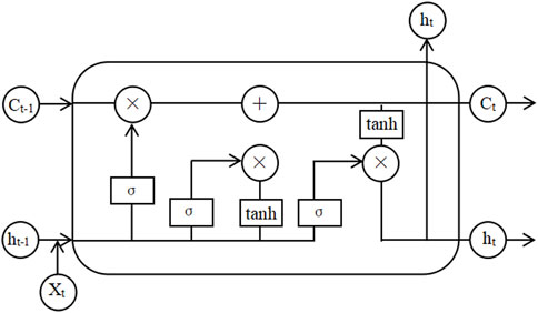
Figure 1. LSTM unit structure diagram.

The forget gate f_t determines whether the information is discarded or retained. The input gate i_t decides to add new information to the current cell state. The output gate o_t determines the final output at time t. The calculation process is shown in the following formula.

${\mathit{f}}_{\mathit{t}}=\mathit{\sigma }\left({\mathit{W}}_{\mathit{f}}·\left[{\mathit{X}}_{\mathit{t}},{\mathit{h}}_{\mathit{t}-\mathbf{1}}\right]+{\mathit{b}}_{\mathit{f}}\right)$

${\mathit{i}}_{\mathit{t}}=\mathit{\sigma }\left({\mathit{W}}_{\mathit{i}}·\left[{\mathit{X}}_{\mathit{t}},{\mathit{h}}_{\mathit{t}-\mathbf{1}}\right]+{\mathit{b}}_{\mathit{i}}\right)$

${\stackrel{\sim }{\mathit{C}}}_{\mathit{t}}=\mathit{tanh}\left({\mathit{W}}_{\mathit{c}}·\left[{\mathit{X}}_{\mathit{t}},{\mathit{h}}_{\mathit{t}-\mathbf{1}}\right]+{\mathit{b}}_{\mathit{c}}\right)$

${\mathit{C}}_{\mathit{t}}={\mathit{f}}_{\mathit{t}}·{\mathit{C}}_{\mathit{t}-\mathbf{1}}+{\mathit{i}}_{\mathit{t}}·{\stackrel{\sim }{\mathit{C}}}_{\mathit{t}}$

${\mathit{o}}_{\mathit{t}}=\mathit{\sigma }\left({\mathit{W}}_{\mathit{o}}·\left[{\mathit{X}}_{\mathit{t}},{\mathit{h}}_{\mathit{t}-\mathbf{1}}\right]+{\mathit{b}}_{\mathit{o}}\right)$

${\mathit{h}}_{\mathit{t}}={\mathit{o}}_{\mathit{t}}·\mathit{tanh}\left({\mathit{C}}_{\mathit{t}}\right)$

Where W represents the weight matrix, b is the bias, σ is the sigmoid activation function, and tanh is the hyperbolic tangent function. X_t is the vector at the t time step of the input sequence, and h_t is the hidden state at the t time step.

3.3 Model explainability methods

3.3.1 SHapley additive exPlanation

SHapley Additive exPlanation (SHAP) is a game theory approach that can be used to interpret the output of any machine learning model. SHAP uses the Shapley value to interpret the predicted value (He et al., 2023) and explore the contribution value of each factor in the prediction. The main idea of this theory is to interpret the predicted value of the model as the sum of the attribute values of each input feature (i.e., the Shapley value), so as to realize the interpretation of the model. The Shapley value is proposed to measure the contribution of multiple people when they collaborate to complete tasks, and its calculation formula is as follows.

$\mathit{V}\left(\mathit{i}\right)={\sum }_{\mathit{S}\subseteq \mathit{N}\backslash \left\{\mathit{i}\right\}}\frac{\left(\left|\mathit{S}\right|!\left(\left|\mathit{N}\right|-\left|\mathit{S}\right|-\mathbf{1}\right)!\right)}{\left|\mathit{N}\right|!}\left(\mathit{v}\left(\mathit{S}\cup \left\{\mathit{i}\right\}\right)-\mathit{v}\left(\mathit{S}\right)\right)$

where $V\left(i\right)$ represents the shapley value of the i-th element, N represents the set of participants, |N| represents the number of elements of the set of participants, S is a subset of N, |S| is the number of subsets of N, and v (S) represents the value of combination S.

Assuming the i-th sample is X_i, the j-th feature of the i-th sample is X_ij, the model’s predicted value for this sample is y_i, and the baseline of the entire model (usually the mean of the target variables of all samples) is y_base, then SHAP value obeys the following equation:

${\mathit{y}}_{\mathit{i}}={\mathit{y}}_{\mathit{b}\mathit{a}\mathit{s}\mathit{e}}+\mathit{f}\left({\mathit{X}}_{\mathit{i}\mathbf{1}}\right)+\mathit{f}\left({\mathit{X}}_{\mathit{i}\mathbf{2}}\right)+...+\mathit{f}\left({\mathit{X}}_{\mathit{i}\mathit{k}}\right)$

where f(X_ij) is the SHAP value of X_i. When f(X_j1)>0, it indicates that this feature improves the predicted value and has a positive effect. Otherwise, it indicates that this feature reduces the predicted value and has a reverse effect.

Traditional feature importance only tells which feature is important, but it is not clear how the feature affects the prediction result. The biggest advantage of SHAP is that it can not only reflect the influence of each feature, but also show the positive and negative effects. In this study, SHAP can be used for the influence of various characteristics on the prediction results of soil temperature prediction model.

3.3.2 Permutation importance

Permutation Importance (PI) can only be used after the model has been trained. It is based on the idea of “replacement test” to detect the importance of features. The permutation importance of each variable is the increase in the mean square error of the model when that variable is randomly shuffled in order (Aldrich, 2020). The more RMSE decreased after a variable was disrupted, the worse the prediction result, indicating that the variable is more important. PI takes into account both the individual effects of each predictor and the multivariable interactions with other predictors. Because the method has certain randomness and instability, the importance of the permutation variables of each feature is appropriate to take the average value of multiple results.

3.3.3 Partial dependence plot

Partial Dependence Plot (PDP) shows the boundary effect of one or two characteristic variables on the model prediction results (Zhang et al., 2023). And it can visualize the relationship between features and predicted outcomes. The basic idea is to select a feature variable, substitute the values of each point in a certain stage, observe the changes of the predicted results, and explore the relationship between the feature and the target feature. In this experiment, we can obtain the relationship between the changes of each characteristic and the predicted results in the prediction of soil temperature by this method. This method is a powerful method to study a single feature.

3.4 Experimental design

This study uses Keras framework for coding based on python3.6. The experimental steps can be divided into four parts: 1. Data set processing 2. Model training 3. Soil temperature prediction 4. Model interpretation. The experimental framework design is shown in Figure 2.

Figure 2

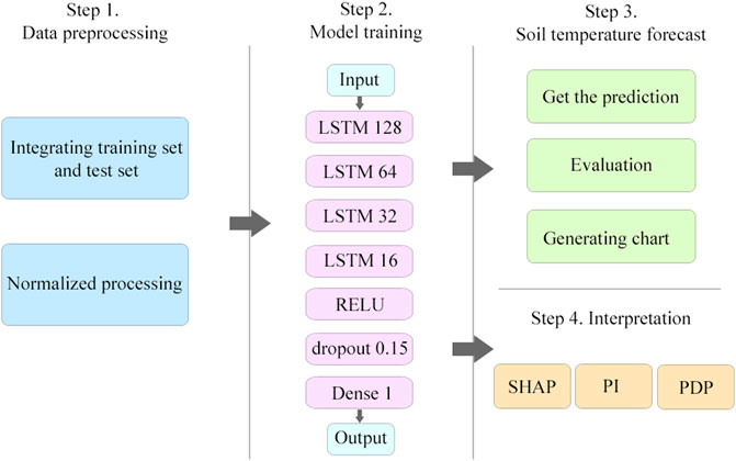
Figure 2. Experiment framework.

First, we process the data set to divide it into the training set and test set that we will use. In this experiment, the training set consists of data from 1990 to 2019, while the test set uses data from 2020. Subsequently, we normalize the data to accelerate convergence.

Figure 2 showcases the architecture of the model, which is structured with four LSTM layers, followed by an activation layer that employs the RELU activation function, and a dropout layer coupled with a fully connected layer for output. We use multiple values for hyper-parameter to perform experiments separately. Finally, the optimal choice is determined as follows. The hidden layer neurons are 128, 64, 32 and 16. The dropout layer is configured with a dropout rate of 0.15 to prevent overfitting. Learning rate is 0.001 and the timestep is 7. The epoch is set to 500.

Besides, the model utilizes the Adam optimizer to achieve swift convergence. RELU is chosen as the activation function because RELU has good robustness, low computational complexity, and no gradient saturation or gradient disappearance (Han et al., 2020). Adding dropout to randomly ignore a certain number of neurons with a specific probability in each training batch can significantly reduce overfitting (Baldi and Sadowski, 2014).

After the training phase, the model’s predictive capabilities were assessed using the test data set. The predicted results are then reverse-normalized for direct comparison with actual soil temperature data. R2, BIAS and RMSE were used to evaluate the performance.

Subsequent to model training, SHAP analysis was conducted to rank the features based on their influence on soil temperature predictions. This offered insights into both general trends and site-specific behaviors. Also, the PI method was applied to corroborate the insights derived from the SHAP analysis.

In the final stage, PDP analysis was performed on individual features to explore their specific relationships with the prediction outcomes. This provided a deeper understanding of how each feature influences the model’s predictions.

The characteristic predicted in this study is soil temperature level 1 (STL1), which means the soil temperature of the first layer (0–7 cm). There are fourteen input variables used, including: air temperature, wind in x-direction, wind in y-direction, precipitation, surface pressure, specific humidity, surface solar radiation, surface thermal radiation, surface net solar radiation, surface net thermal radiation, sensible heat flux, latent heat flux, DEM, land type. DEM and land type are two static variables. Explanations and abbreviations of all these variables are added to the table in the Appendix. Abbreviations are used in the figures.

4 Results

4.1 Model performance evaluation

R2, bias and RMSE were used as evaluation indicators in this experiment.

R2 is the coefficient of determination, and its formula can be expressed as.

$\mathit{R}\mathbf{2}=\mathbf{1}-\frac{{\displaystyle \sum _{\mathit{i}}}{\left(\widehat{{\mathit{y}}_{\mathit{i}}}-{\mathit{y}}_{\mathit{i}}\right)}^{\mathbf{2}}}{{\displaystyle \sum _{\mathit{i}}}{\left(\overline{{\mathit{y}}_{\mathit{i}}}-{\mathit{y}}_{\mathit{i}}\right)}^{\mathbf{2}}}$

Where y represents the actual value, $\overline{y}$ represents the average of the actual value, and $\widehat{y}$ represents the predicted value. The model is judged according to the value of R2. Its value range is [0,1]. The closer the value is to 1, the better the model performance is bias indicates the average of the absolute value of the difference between the true value and the predicted value. A smaller value indicates better performance.

RMSE is the mean square error root, which is the mean opening root of the sum of squares of the difference between the data and the true value, that is, the mean of the sum of squares of errors. The smaller the RMSE, the higher the measurement accuracy.

The formula is expressed as:

$\mathit{R}\mathit{M}\mathit{S}\mathit{E}=\sqrt{\frac{{\sum }_{\mathit{i}=\mathbf{1}}^{\mathit{N}}{\left({\mathit{y}}_{\mathit{i}}-\widehat{{\mathit{y}}_{\mathit{i}}}\right)}^{\mathbf{2}}}{\mathit{N}}}$

Finally, the R of the model is 0.89, R2 is 0.7, RMSE is 2.4, and bias is 2.0.

Figure 3A shows the predicted soil temperature 1 day later using the model, and Figure 3B shows the actual measurement results.

Figure 3

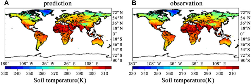
Figure 3. Comparison of model predicted value distribution (A) and true value (B).

In order to prove the applicability of LSTM in the field of soil temperature prediction, we choose Backpropagation Neural Network (BPNN) and Support Vector Regression (SVR) as the benchmark model.

BPNN is the most widely used neural network at present. It consists of an input layer, a hidden layer and an output layer. The layers are completely connected to each other, and there is no connection between the same layer. It had a learning rate of 0.001 and 128 hidden layer neurons using the Adam optimizer. Support Vector Machine (SVM) is a commonly used supervised learning algorithm. It is mainly used for classification and regression problems. Based on the idea of structural risk minimization, the classification or regression task is realized by finding an optimal hyperplane in the feature space. SVR is the application of SVM to regression problems. In this experiment, the kernal is selected as ‘rbf’, which has the advantages of high efficiency and few parameters.

For LSTM, BPNN, and SVR, we use the same training set and test set, using RMSE as a metric to compare their performance. The result is shown in Figure 4.

Figure 4

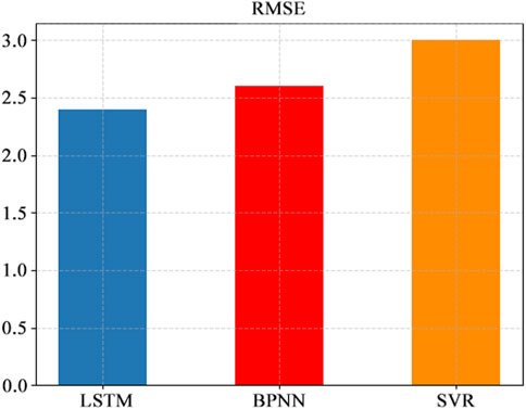
Figure 4. RMSE of LSTM, BPNN and SVR

When predicting soil temperature, the RMSE of LSTM was 0.2 lower than that of BPNN and 1.6 lower than that of SVR. The results show that compared with BPNN and SVR, LSTM neural network model has lower error and higher precision in soil temperature time series prediction. LSTM is more suitable for soil temperature prediction.

At the same time, we tried to add the first three layers of soil temperature STL1, soil temperature level 2 (STL2) and soil temperature level 3 (STL3) into the input variables, and the model performance was better. Its R value is 0.90 and R2 is 0.94. The comparison is shown in Figure 5, (a) is the predicted value of soil temperature, (b) is the actual value of soil temperature, red represents high temperature, blue represents low temperature, unit is Kelvin (K).

Figure 5

Figure 5. Compares the predicted value distribution (A) of the model with the actual value (B) after STL1, STL2, and STL3 are added to the input.

In our continued interpretation, we discovered that soil temperature exhibits a high level of stability. Of all the factors impacting soil temperature prediction, its own influence is the most significant. The inclusion of STL1, STL2, and STL3 as input variables greatly outweighs the influence of all other variables, making it challenging to discern the effects of the other variables. As a result, this study will concentrate on the model excluding STL1, STL2, and STL3, with the interpretation of results after their inclusion provided in the subsequent paragraphs.

4.2 Comparative analysis of results from SHAP and PI

This section uses a summary plot to sort the importance of global features with positive and negative impacts, based on the SHAP method. After conducting numerous experiments, all geographical coordinates across the globe were systematically sampled. The findings are illustrated in Figure 6.

Figure 6

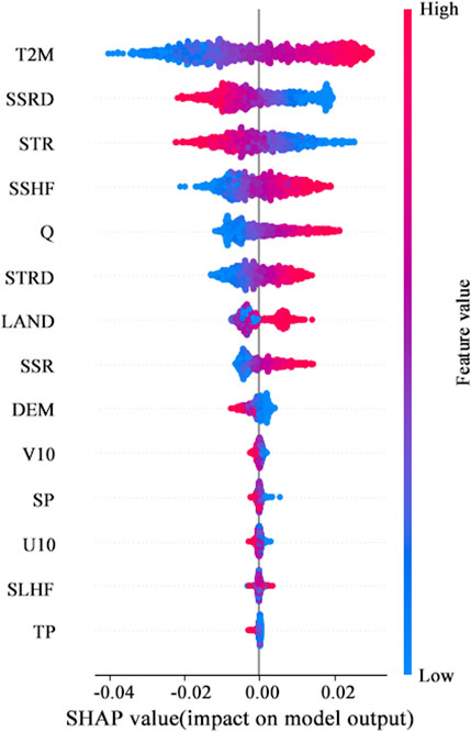
Figure 6. Feature importance ranking and positive and negative impact summary.

In Figure 6, the color of the shadow represents the size of the feature value. The closer to red, the larger the value, and the closer to blue, the smaller the value. The position of each feature on the graph is sorted according to the absolute value of all the SHAP values of the feature from largest to smallest. The higher the position is, the more important the feature is.

Among the variables we analyzed, air temperature emerged as the most critical forcing variable. Its PI value in predicting soil temperature aligns with expectations, given the interdependent relationship between air temperature and soil temperature. It shows air temperature an indispensable factor. Following closely are variables such as surface solar radiation, surface net thermal radiation, and sensible heat flux, highlighting their significant but lesser roles. Static variables like land type and DEM are positioned at 7th and 9th in terms of importance, respectively. This ranking suggests that soil type and terrain, while relevant, exert a relatively modest impact on soil temperature dynamics. Conversely, variables related to wind speed (wind in x-direction and wind in y-direction), precipitation, latent heat flux, and surface pressure rank low in importance. Their minimal influence on the predictive outcomes underscores their peripheral role in soil temperature forecasting.

Using the variable air temperature, which holds the highest significance, as an illustration, the more intense the red hue, signifying a higher feature value, the greater the corresponding SHAP value. Conversely, a shift towards blue signifies a lower feature value, correlating with a decrease in the SHAP value, sometimes extending into negative territory. It underscores a positive correlation between soil temperature predictions and air temperature. As air temperature increases, so does the soil temperature, with both positive and negative impacts being markedly pronounced.

In contrast, for surface solar radiation, an increase in its feature value leads to a rise in the SHAP value, while a decrease in the feature value results in a lower SHAP value. This suggests a negative correlation with soil temperature, a trend similarly observed with surface net thermal radiation, which also exhibits a significant negative correlation. Conversely, variables like sensible heat flux, specific humidity, and surface thermal radiation demonstrate a positive correlation with soil temperature predictions. Specifically, a higher feature value in specific humidity amplifies the positive correlation with the prediction outcomes. However, a decrease in the feature value results in a less pronounced drop in the SHAP value, indicating that the negative impacts are less significant.

In 2005, Hu and Feng (2005) proved that there was a strong positive correlation between surface air temperature and surface soil temperature, and a weak correlation between precipitation and surface soil temperature. This is consistent with our interpretation.

Additionally, we chose four distinct locations across the globe and extracted their SHAP values for comparative analysis alongside the global findings. These locales encompass Greenland, renowned for its perpetual coldness and vast ice-covered landscapes; the Tibetan Plateau, distinguished as the world’s highest plateau, subjected to intense solar radiation; the Nicaraguan Plain, characterized by its sweltering heat and frequent rainfall; and Chad, situated in central Africa, experiencing a scorching and arid climate. These diverse geographical and climatic settings make these locations highly representative on a global scale. We chose these to examine their individual feature importance rankings, aiming to ascertain whether the outcomes depicted in Figure 6 would undergo substantial alterations under various, more extreme scenarios. Figure 7 presents the outcomes for various geographical points: (a) corresponds to a location pinpointed on (e) within Greenland; (b) represents results from a specific point on the Tibetan Plateau, identified on (f); (c) showcases outcomes for a point in Nicaragua, designated on (g); (d) illustrates results for a point in Chad, marked on (h).

Figure 7

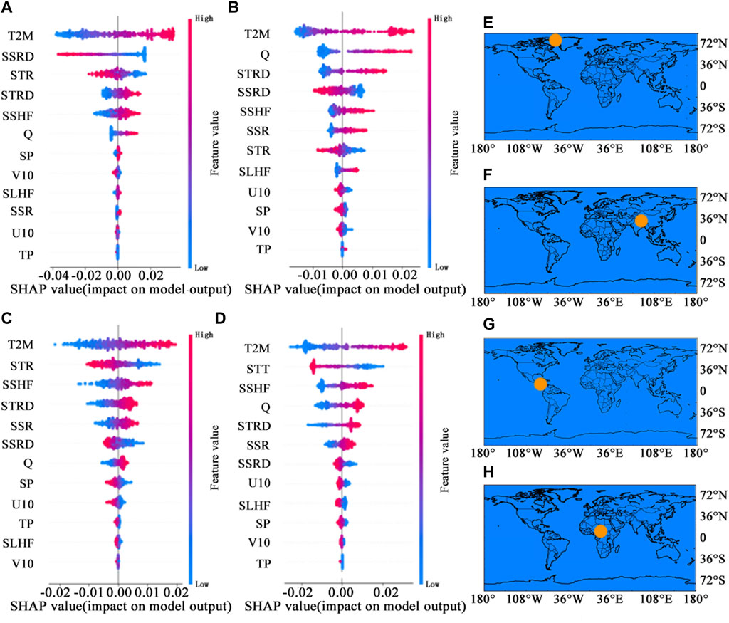
Figure 7. Feature importance ranking and positive and negative impacts summary of some locations.

The results show that the ranking of variable importance in these regions is consistent with global trends, with air temperature consistently holding the top position with significant advantage. The order of the next six features—surface solar radiation, surface net thermal radiation, surface net solar radiation, sensible heat flux, specific humidity, and surface thermal radiation—experiences minor variations but they consistently remain within the top seven, alongside air temperature. Surface thermal radiation emerges as the second most important variable in the majority of the sites. The positive or negative correlations associated with each feature also display consistency across different global locations. Due to the static nature of the variables DEM and land type, which maintain consistent values at every time point within the same location, it becomes impossible to generate SHAP charts for them. Consequently, these variables fall outside the purview of this research.

In predicting soil temperature in Greenland, when the surface solar radiation characteristic value is high, its SHAP value becomes negative and falls below the average level. Moreover, in other regions, it exerts a more prominent negative influence on soil temperature prediction. The topography of the Qinghai-Tibet Plateau is intricate, and for illustrative purposes, we focus on a specific point. At this location, only the SHAP value of specific humidity aligns with the global scope, while the SHAP ranges of other mean eigenvalues are narrower than the global extent. Nicaragua resides in central Central America, where the climate is notably shaped by oceanic influences. Notably, wind in y-direction holds greater importance than wind in x-direction, while the remaining factors show no significant deviation from the global average. Chad, situated in central Africa, has a higher impact on the forecast than wind in y-direction.

The principles and calculation methods of PI and SHAP may differ, yet both approaches yield feature importance rankings. To determine the significance of each feature, we assessed the RMSE difference by reshuffling the order of features. Given that PI exhibits more randomness and instability compared to SHAP, we derived the average RMSE from multiple iterations of the shuffled results.

As illustrated in Figure 8, there was a notable change in the RMSE of the predicted results before and after the disruption of air temperature. This alteration underscores the substantial impact this variable holds on the model’s soil temperature predictions.

Figure 8

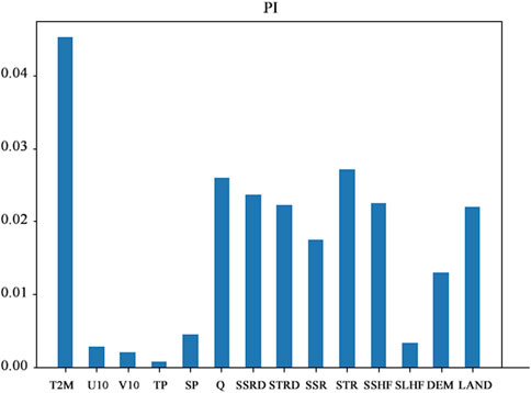
Figure 8. Feature importance from PI.

Consistent with the global SHAP outcomes depicted in Figure 6, air temperature features emerge as the most crucial, followed by other variables in a slightly different sequence, yet generally aligned. Notably, wind in x-direction, wind in y-direction, precipitation, surface pressure, and latent heat flux appear to have lower importance, ranking towards the bottom in both interpretation methods. The interpretation outcomes of PI and SHAP can be cross-validated to reinforce their credibility.

To explore the relationship between various features and soil temperature, we selected six global land points and randomly chose 100 days’ worth of data from the validation set, which included air temperature, precipitation, and soil temperature. Utilizing SHAP and PI methods, we found that air temperature significantly influences soil temperature variations, whereas precipitation has a minimal impact. Figure 9 illustrates the correlation between air temperature, precipitation, and the actual soil temperature values. In this figure, the blue line denotes air temperature, the red line represents precipitation, and the orange line indicates soil temperature. It is evident that soil temperature and air temperature exhibit a clear, consistent trend, whereas the variations of precipitation appear relatively independent, showing no significant correlation with soil temperature. This observation confirms that our model’s interpretation through SHAP and PI accurately mirrors real-world dynamics.

Figure 9

Figure 9. Relationship between soil temperature and air temperature and precipitation.

We can also obtain the distribution of various features in different places around the world at different times through SHAP. The SHAP value of the same feature is not only different at each coordinate point, but also has different SHAP value at different periods for the same coordinate point. Figure 10 shows the distribution of SHAP values of characteristic air temperature in different periods in 2020, with a interval of 30 days between each two graphs. It can be clearly seen from the figure (a), (b) and (c) that SHAP values in the northern hemisphere are mostly negative, while those in the Southern Hemisphere are mostly positive, (d) (e) is a transition state, and the changes in the northern hemisphere in (f), (g), (h) and (i) are mostly positive, while most of the SHAP values in the Southern Hemisphere are negative. After the transition of the two figures (j) and (k) again, the (L) figure returns to a state where the northern hemisphere is negative and the southern hemisphere is positive. From the 12 graphs, we can see that the SHAP distribution of air temperature has obvious timing.

Figure 10

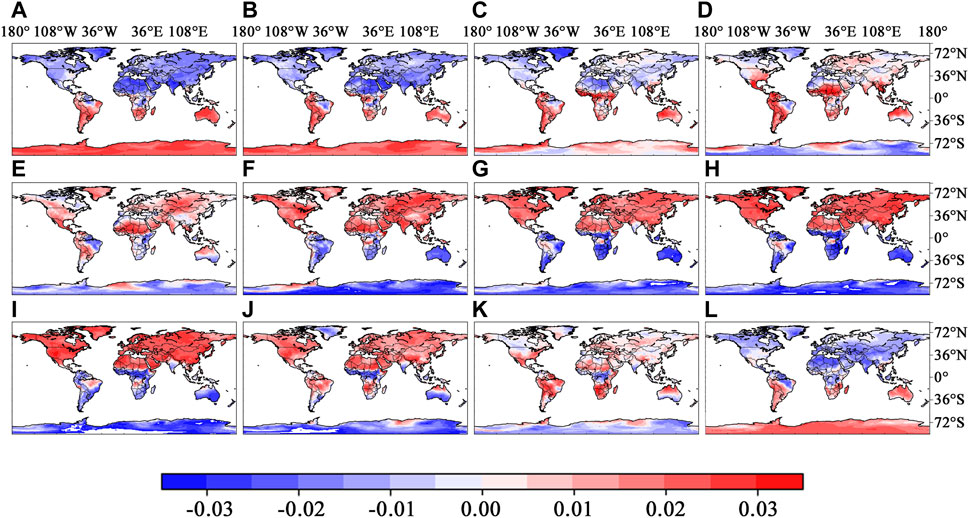
Figure 10. SHAP values of air temperature at different periods in 2020.

SHAP analysis also enables us to discern the distribution of various features across different global locations and times. The SHAP value for a single feature not only varies across geographical coordinates but also fluctuates over different periods at the same location. Figure 10 depicts the temporal distribution of SHAP values for the feature air temperature throughout 2020, with each graph spaced 30 days apart. From figures (a), (b), and (c), it is apparent that SHAP values are predominantly negative in the Northern Hemisphere and positive in the Southern Hemisphere. Figures (d) and (e) represent transitional states, with the Northern Hemisphere shifting to mostly positive SHAP values in figures (f) through (i), while the Southern Hemisphere exhibits mostly negative values. After another transition in figures (j) and (k), figure (L) shows a return to the initial state with negative values in the Northern Hemisphere and positive in the Southern Hemisphere. This cyclical pattern across the 12 graphs highlights the temporal nature of air temperature’s SHAP distribution. Figures (a), (b), and (c) correspond to the Northern Hemisphere’s winter months, where air temperature’s characteristic values are low, leading to negative SHAP values. This suggests that air temperature significantly lowers the model’s soil temperature predictions during this period. Conversely, during the Northern Hemisphere’s summer months, as seen in figures (f) through (i), air temperature’s values are high, and its SHAP values are positive, indicating an amplifying effect on soil temperature predictions.

Figure 11 explores the distribution of the feature surface solar radiation, showcasing significant seasonal impacts in the Northern Hemisphere and Antarctica. During the Northern Hemisphere’s winter, SHAP values are mostly positive, contrasting with negative values in Antarctica. As temperatures rise in the Northern Hemisphere, SHAP values shift to negative, then to positive in Antarctica, reflecting a seasonal inversion. By the end of summer, this pattern reverses again. However, regions in the Southern Hemisphere, excluding Antarctica, display no clear temporal pattern, with consistently negative SHAP values throughout this season.

Figure 11

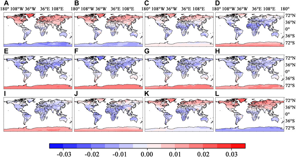
Figure 11. SHAP values of surface solar radiation at different periods in 2020.

4.3 Result analysis of PDP

PDP is an explainable method for the study of a single feature. For the convenience of observation, we put multiple examples on the same chart and take their average values to show them in the red line, as shown in Figure 12. Figure 12 shows how the predicted soil temperature results change as one variable increases. The horizontal axis is the value of each variable, and the vertical axis is the predicted value of soil temperature. The data of both have been normalized. The green line represents the change in each instance, and here we have 500 examples, each of which has 500 green lines. The red line is the value we obtained by taking the average of 500 values, showing the overall trend of the influence of this feature change on the result prediction. The obvious increase indicates that the feature is positively correlated with soil temperature, while the obvious decrease indicates that the feature is negatively correlated with soil temperature.

Figure 12

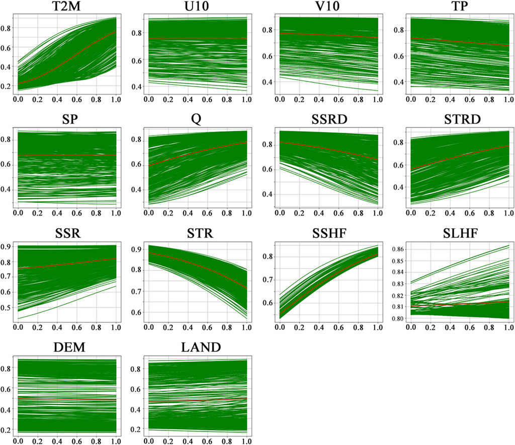
Figure 12. PDP of soil temperature prediction.

PDP offer an interpretable technique for analyzing the impact of individual features. For clarity, we overlay multiple instances on a single chart and depict their average with a red line, as illustrated in Figure 12. This figure demonstrates the variation in predicted soil temperature as a function of a single variable’s increase. The horizontal axis represents the values of the variable in question, while the vertical axis shows the corresponding predicted soil temperatures, with both sets of data normalized for comparison. The green lines trace the changes for each instance, with a total of 500 examples, resulting in an equal number of green lines. The red line, derived from averaging these 500 values, reveals the general trend of how changes in this feature affect prediction outcomes. A noticeable uptick suggests a positive correlation with soil temperature, whereas a clear downtrend indicates a negative correlation.

Among the variables, air temperature exhibits the strongest positive correlation, significantly driving up soil temperature as it increases, with the rate of increase accelerating. This makes air temperature the feature most closely associated with soil temperature predictions. Other variables, including specific humidity, sensible heat flux, surface thermal radiation, surface net solar radiation, and another instance of sensible heat flux, show a similar pattern to air temperature, where the predicted soil temperature rises alongside increases in these variables. Conversely, surface solar radiation and surface net thermal radiation are observed to lower the predicted soil temperature as they increase. Meanwhile, wind in x-direction, wind in y-direction, precipitation, surface pressure, latent heat flux, and the two static variables, DEM and land type, exert minimal influence on the prediction outcomes, with the predicted values remaining largely unchanged throughout their variations. When juxtaposed with the SHAP analysis, it becomes evident that features critical to soil temperature prediction manifest pronounced trends of increase or decrease on the PDP chart. In contrast, features with negligible impact on predictions display almost flat lines, underscoring their limited influence.

5 Discussion

This research employs a multi-layer LSTM model to forecast soil temperature, utilizing the dataset from the LandBench toolbox spanning from 1990 to 2019 for training, and data from 2020 for testing. The findings reveal the potential of deep learning in soil temperature prediction. Notably, soil temperature was deliberately excluded from the model’s input variables to sharpen the focus of the study. Contrary to the conventional belief that deep learning models must trade off explainability for predictive accuracy, our study dispels this myth by showing that it is feasible to excel in both areas simultaneously. Despite the model’s strong predictive performance, we delved into its explainability through SHAP and other methods. This not only laid a robust foundation for understanding the model’s predictions but also significantly improved its fairness and transparency.

Integrating explainability techniques into deep learning models enhances their practical utility and facilitates their broader adoption across various fields. This integration is instrumental in continuously improving model performance. Consequently, deep learning models become a powerful tool, offering critical insights into agriculture, earth sciences, and beyond, representing a substantial advancement in their application.

To interpret the model, we employed SHAP and PI methodologies to assess the influence of each predictor on the model’s output, identifying whether they increase or decrease the predicted results. PDP were used to explore the relationship between individual variables and the prediction outcomes over a range of values, providing a nuanced understanding of how each feature contributes to the model’s predictions.

Upon applying the explainability technique SHAP, it becomes evident that air temperature is the most significant predictor. Its predominant influence over other variables aligns with expectations, underscoring the substantial effect of air temperature on soil temperature. Following air temperature, surface solar radiation and surface net thermal radiation emerge as crucial factors. The quartet of radiation variables—encompassing both long and short wave radiation, alongside their respective downward and upward differences—exerts a notable impact. Conversely, the contributions of the two wind components, surface pressure, and precipitation are comparatively modest. The study also incorporates two static variables, land type and DEM, as input variables. However, their impact on the prediction outcomes is relatively minor.

This conclusion is corroborated by alternative methodologies as well. Within the feature importance rankings derived via the PI method, air temperature emerges as a standout, exerting the most substantial impact on prediction outcomes, with other features aligning closely with SHAP analysis results.

By analyzing the SHAP summary plot, it becomes evident that air temperature, sensible heat flux, specific humidity, surface thermal radiation, land type, and surface net solar radiation have a strong positive correlation with the prediction outcomes. This means that as their eigenvalues increase, so does the magnitude of the prediction results. Conversely, surface solar radiation and surface net thermal radiation exhibit a marked negative correlation with the predictive outcomes, indicating that larger eigenvalues lead to a diminished influence on the prediction results.

Furthermore, we leveraged the PDP to assess how variations in a single variable affect the predicted outcomes, corroborating these findings with the SHAP summary plot. Utilizing the PDP method, we analyzed over 500 examples from locations worldwide. The analysis revealed that higher-ranked features exhibit more consistent PDP curves, whereas lower-ranked features display more variability, lacking in regularity, with flatter curves.

Notably, the PDP plot for air temperature generally shows an upward trajectory, particularly demonstrating a sharp increase in the predicted outcome as the eigenvalue grows beyond a positive threshold. This trend aligns with the observations from the SHAP cellular graph, where variables exhibiting a positive correlation in the SHAP plot, such as sensible heat flux, similarly show an upward trend in the PDP plot. Conversely, variables with a negative correlation in the SHAP plot, like surface thermal radiation, exhibit a downward trend in the PDP plot.

Moreover, the ranking of feature importance varies slightly across different geographical coordinates. For instance, the impact of specific humidity on the predicted outcomes in a location of the Tibetan Plateau is significantly higher than the global average. Meanwhile, the influence of surface solar radiation on predictions in a location of Chad, Central Africa, is notably lower.

The SHAP values for certain features exhibit clear seasonal patterns throughout the year, with the air temperature characteristic being the most pronounced. This feature typically shows a positive SHAP value during the high temperatures of summer and a negative value during the low temperatures of winter. Specifically, in winter, the SHAP values for air temperature in regions like Greenland, northern Africa, and the Arabian Peninsula are notably lower compared to other areas. These values gradually increase and then sharply decrease in Greenland and Antarctica with the changing seasons, a phenomenon that is intricately linked to the extensive ice and snow coverage in these regions.

We also conducted an additional supplementary experiment. In this experiment, we incorporated soil temperatures (STL1, STL2, and STL3) as input variables and utilized data from the preceding 7 days to forecast the soil temperature on the eighth day. The findings indicate that these three variables are pivotal in predicting soil temperature, with STL1 and STL2 (covering soil depths of 0–28 cm) being particularly critical. As illustrated in Figure 13, STL1 and STL2 significantly outperform other variables in terms of predictive power, whereas STL3 exhibits a marginally lesser impact compared to air temperature. The ranking of the remaining variables remains largely consistent.

Figure 13

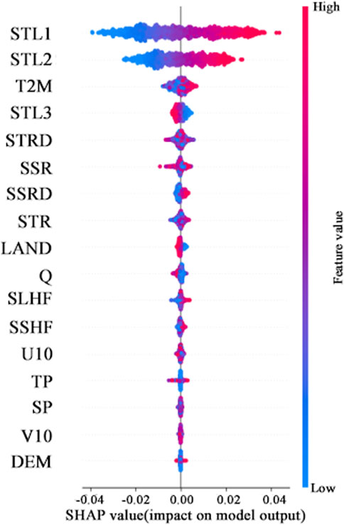
Figure 13. Feature importance ranking and positive and negative impacts summary after adding STL1, STL2 and STL3 into input.

6 Conclusion

This study introduces an interpretable multi-layer LSTM model designed for predicting global soil temperatures, leveraging SHAP, PI, and PDP methodologies for explanatory analysis. The main conclusions can be summarized as follows: the application of multiple explainability methods yielded consistent results, validating the applicability of XAI in soil temperature prediction, particularly in conjunction with LSTM models.

Our research utilized fourteen input variables, including two static ones: DEM and land type. It was discovered that the variable exerting the most significant influence on soil temperature prediction is air temperature, whose SHAP values and PI feature values demonstrate notable seasonality. As well, four radiation variables (surface solar radiation, surface thermal radiation, surface net solar radiation and surface net thermal radiation) were found to impact the prediction outcomes to a certain extent, whereas the influence of the two static variables (land type and DEM) was comparatively minor. Other variables such as total precipitation, wind speed (wind in x-direction and wind in y-direction), surface pressure and latent heat flux had a negligible effect on soil temperature. The study underscores temperature and radiation as the primary determinants of soil temperature. Moreover, incorporating soil temperature variables (STL1 and STL2) into the input significantly affected the prediction, particularly the temperatures of the soil’s surface layer (0–7 cm) and the subsequent layer (7–28 cm).

The employment of SHAP, PI, and PDP methods yielded consistent results across the board. SHAP and PI provided global explanations, ranking the importance of the input variables and consistently highlighting the significant role of air temperature. SHAP, in particular, not only ranked the variables by importance but also intuitively depicted the directional impact of each feature’s values on the prediction outcome, allowing for inferences about positive or negative correlations with the prediction target. PDP illustrated the relationship between specific features and the prediction target by varying a feature’s value. A comparison between SHAP and PDP results demonstrated mutual corroboration, for instance, indicating a positive correlation between air temperature and soil temperature, while surface solar radiation and surface net thermal radiation showed negative correlations, aligning with empirical observations.

The explanatory insights provided in this paper enhance the transparency and credibility of the model, enabling users to grasp the underlying predictive mechanisms. Research on the applicability of XAI can help developers improve the performance of soil temperature prediction models and can promote the recognition and acceptance of deep learning in the field of soil temperature prediction. By knowing its internal principles, the market can easily establish a supervision system for applications based on deep learning, which also lays the foundation for a broader and safer application of deep learning in the future. Overall, this study demonstrates the potential of XAI in elucidating deep learning models, particularly in soil temperature prediction, underscoring its importance for practical deployment and application of deep learning.

This study also has some shortcomings. Firstly, this study only reflects the influence of each feature on the result, and does not reflect the interaction between the features. At present, there is no interpretable method to show the interaction between more than two features at the same time, and this will be a problem that needs to be solved in the future. Secondly, the current research on explainability mainly focuses on Post-hoc methods, mainly SHAP, and the Intrinsic methods are relatively limited. It is hoped that more efficient and accurate explainability methods can be developed in the future.

Data availability statement

The data analyzed in this study is subject to the following licenses/restrictions: Data available on request due to privacy. Requests to access these datasets should be directed to QL, [email protected].

Author contributions

QG: Writing–review and editing, Project administration, Methodology, Formal Analysis, Conceptualization. LW: Writing–original draft, Visualization, Software, Methodology, Investigation. QL: Writing–review and editing, Validation, Supervision, Resources, Funding acquisition, Data curation.

Finanzierung

The author(s) declare that financial support was received for the research, authorship, and/or publication of this article. The study was partially supported by the Jilin Provincial Science and Technology Development Plan Project under grants 20230101370J.

Conflict of interest

The authors declare that the research was conducted in the absence of any commercial or financial relationships that could be construed as a potential conflict of interest.

Publisher’s note

All claims expressed in this article are solely those of the authors and do not necessarily represent those of their affiliated organizations, or those of the publisher, the editors and the reviewers. Any product that may be evaluated in this article, or claim that may be made by its manufacturer, is not guaranteed or endorsed by the publisher.

References

Aldrich, C. (2020). Process variable importance analysis by use of random forests in a shapley regression framework. Minerals 10 (5), 420. doi:10.3390/min10050420

CrossRef Full Text | Google Scholar

Alizamir, M., Kisi, O., Ahmed, A. N., Mert, C., Fai, C. M., Kim, S., et al. (2020). Advanced machine learning model for better prediction accuracy of soil temperature at different depths. PLoS One 15 (4), e0231055. doi:10.1371/journal.pone.0231055

PubMed Abstract | CrossRef Full Text | Google Scholar

Arrieta, A. B., Díaz-Rodríguez, N., Del Ser, J., Bennetot, A., Tabik, S., Barbado, A., et al. (2020). Explainable Artificial Intelligence (XAI): concepts, taxonomies, opportunities and challenges toward responsible AI. Inf. fusion 58, 82–115. doi:10.1016/j.inffus.2019.12.012

CrossRef Full Text | Google Scholar

Baldi, P., and Sadowski, P. (2014). The dropout learning algorithm. Artif. Intell. 210, 78–122. doi:10.1016/j.artint.2014.02.004

PubMed Abstract | CrossRef Full Text | Google Scholar

Bilgili, M. (2010). Prediction of soil temperature using regression and artificial neural network models. Meteorology Atmos. Phys. 110, 59–70. doi:10.1007/s00703-010-0104-x

CrossRef Full Text | Google Scholar

Chen, G., Li, L., Zhang, Z., and Li, S. (2020). Short-term wind speed forecasting with principle-subordinate predictor based on Conv-LSTM and improved BPNN. IEEE Access 8, 67955–67973. doi:10.1109/ACCESS.2020.2982839

CrossRef Full Text | Google Scholar

Chen, Q., Mao, P., Zhu, S., Xu, X., and Feng, H. (2024). A decision-aid system for subway microenvironment health risk intervention based on backpropagation neural network and permutation feature importance method. Build. Environ. 253, 111292. doi:10.1016/j.buildenv.2024.111292

CrossRef Full Text | Google Scholar

Chen, Z., Zhu, Z., Jiang, H., and Sun, S. (2020). Estimating daily reference evapotranspiration based on limited meteorological data using deep learning and classical machine learning methods. J. Hydrology 591, 125286. doi:10.1016/j.jhydrol.2020.125286

CrossRef Full Text | Google Scholar

Datta, P., and Faroughi, S. A. (2023). A multihead LSTM technique for prognostic prediction of soil moisture. Geoderma 433, 116452. doi:10.1016/j.geoderma.2023.116452

CrossRef Full Text | Google Scholar

Delbari, M., Sharifazari, S., and Mohammadi, E. (2019). Modeling daily soil temperature over diverse climate conditions in Iran—a comparison of multiple linear regression and support vector regression techniques. Theor. Appl. Climatol. 135, 991–1001. doi:10.1007/s00704-018-2370-3

CrossRef Full Text | Google Scholar

Delhasse, A., Kittel, C., Amory, C., Hofer, S., van As, D., S. Fausto, R., et al. (2020). Brief communication: evaluation of the near-surface climate in ERA5 over the Greenland ice sheet. Cryosphere 14 (3), 957–965. doi:10.5194/tc-14-957-2020

CrossRef Full Text | Google Scholar

ElSaadani, M., Habib, E., Abdelhameed, A. M., and Bayoumi, M. (2021). Assessment of a spatiotemporal deep learning approach for soil moisture prediction and filling the gaps in between soil moisture observations. Front. Artif. Intell. 4, 636234. doi:10.3389/frai.2021.636234

PubMed Abstract | CrossRef Full Text | Google Scholar

Friedl, M. A., Sulla-Menashe, D., Tan, B., Schneider, A., Ramankutty, N., Sibley, A., et al. (2010). MODIS Collection 5 global land cover: algorithm refinements and characterization of new datasets. Remote Sens. Environ. 114 (1), 168–182. doi:10.1016/j.rse.2009.08.016

CrossRef Full Text | Google Scholar

Gupta, L. K., Koundal, D., and Mongia, S. (2023). Explainable methods for image-based deep learning: a review. Archives Comput. Methods Eng. 30 (4), 2651–2666. doi:10.1007/s11831-023-09881-5

CrossRef Full Text | Google Scholar

Han, Z., Yu, S., Lin, S. B., and Zhou, D. X. (2020). Depth selection for deep ReLU nets in feature extraction and generalization. IEEE Trans. Pattern Analysis Mach. Intell. 44 (4), 1853–1868. doi:10.1109/TPAMI.2020.3032422

PubMed Abstract | CrossRef Full Text | Google Scholar

Hao, H., Yu, F., and Li, Q. (2020). Soil temperature prediction using convolutional neural network based on ensemble empirical mode decomposition. IEEE Access 9, 4084–4096. doi:10.1109/ACCESS.2020.3048028

CrossRef Full Text | Google Scholar

He, Z., Yang, Y., Fang, R., Zhou, S., Zhao, W., Bai, Y., et al. (2023). Integration of Shapley additive explanations with random forest model for quantitative precipitation estimation of mesoscale convective systems. Front. Environ. Sci. 10, 1057081. doi:10.3389/fenvs.2022.1057081

CrossRef Full Text | Google Scholar

Hu, Q., and Feng, S. (2005). How have soil temperatures been affected by the surface temperature and precipitation in the Eurasian continent? Geophys. Res. Lett. 32 (14). doi:10.1029/2005GL023469

CrossRef Full Text | Google Scholar

Jena, R., Pradhan, B., Gite, S., Alamri, A., and Park, H. J. (2023). A new method to promptly evaluate spatial earthquake probability mapping using an explainable artificial intelligence (XAI) model. Gondwana Res. 123, 54–67. doi:10.1016/j.gr.2022.10.003

CrossRef Full Text | Google Scholar

Jiang, P., Liu, Z., Abedin, M. Z., Wang, J., Yang, W., and Dong, Q. (2024). Profit-driven weighted classifier with interpretable ability for customer churn prediction. Omega 125, 103034. doi:10.1016/j.omega.2024.103034

CrossRef Full Text | Google Scholar

Kim, B., Park, J., and Suh, J. (2020). Transparency and accountability in AI decision support: explaining and visualizing convolutional neural networks for text information. Decis. Support Syst. 134, 113302. doi:10.1016/j.dss.2020.113302

CrossRef Full Text | Google Scholar

Lee, S., and Yoo, S. (2024). InterDILI: interpretable prediction of drug-induced liver injury through permutation feature importance and attention mechanism. J. Cheminformatics 16 (1), 1. doi:10.1186/s13321-023-00796-8

CrossRef Full Text | Google Scholar

Li, H., Vulova, S., Rocha, A. D., and Kleinschmit, B. (2024a). Spatio-temporal feature attribution of European summer wildfires with Explainable Artificial Intelligence (XAI). Sci. Total Environ. 916, 170330. doi:10.1016/j.scitotenv.2024.170330

PubMed Abstract | CrossRef Full Text | Google Scholar

Li, Q., et al. (2022). An attention-aware LSTM model for soil moisture and soil temperature prediction. Geoderma 409, 115651. doi:10.1016/j.eswa.2023.122917

CrossRef Full Text | Google Scholar

Li, Q., Zhang, C., Shangguan, W., Wei, Z., Yuan, H., Zhu, J., et al. (2024b). LandBench 1.0: a benchmark dataset and evaluation metrics for data-driven land surface variables prediction. Expert Syst. Appl. 243, 122917. doi:10.1016/j.eswa.2023.122917

CrossRef Full Text | Google Scholar

Liu, Z., Jiang, P., Wang, J., Du, Z., Niu, X., and Zhang, L. (2023). Hospitality order cancellation prediction from a profit-driven perspective. Int. J. Contemp. Hosp. Manag. 35 (6), 2084–2112. doi:10.1108/ijchm-06-2022-0737

CrossRef Full Text | Google Scholar

Miao, K., Houssou Hounye, A., Su, L., Pan, Q., Wang, J., Hou, M., et al. (2024). Exploring explainable machine learning and Shapley additive exPlanations (SHAP) technique to uncover key factors of HNSC cancer: an analysis of the best practices. Biomed. Signal Process. Control 89, 105752. doi:10.1016/j.bspc.2023.105752

CrossRef Full Text | Google Scholar

Mihalakakou, G. (2002). On estimating soil surface temperature profiles. Energy Build. 34 (3), 251–259. doi:10.1016/S0378-7788(01)00089-5

CrossRef Full Text | Google Scholar

Naga Srinivasu, P., Ijaz, M. F., and Woźniak, M. (2024). XAI-driven model for crop recommender system for use in precision agriculture. Comput. Intell. 40 (1), e12629. doi:10.1111/coin.12629

CrossRef Full Text | Google Scholar

Palazzolo, N., Peres, D. J., Creaco, E., and Cancelliere, A. (2023). Using principal component analysis to incorporate multi-layer soil moisture information in hydrometeorological thresholds for landslide prediction: an investigation based on ERA5-Land reanalysis data. Nat. Hazards Earth Syst. Sci. 23 (1), 279–291. doi:10.5194/nhess-23-279-2023

CrossRef Full Text | Google Scholar

Paul, K. I., Polglase, P. J., Smethurst, P. J., O’Connell, A. M., Carlyle, C. J., and Khanna, P. K. (2004). Soil temperature under forests: a simple model for predicting soil temperature under a range of forest types. Agric. For. Meteorology 121 (3-4), 167–182. doi:10.1016/j.agrformet.2003.08.030

CrossRef Full Text | Google Scholar

Saeed, W., and Omlin, C. (2023). Explainable AI (XAI): a systematic meta-survey of current challenges and future opportunities. Knowledge-Based Syst. 263, 110273. doi:10.1016/j.knosys.2023.110273

CrossRef Full Text | Google Scholar

Samadianfard, S., Asadi, E., Jarhan, S., Kazemi, H., Kheshtgar, S., Kisi, O., et al. (2018). Wavelet neural networks and gene expression programming models to predict short-term soil temperature at different depths. Soil Tillage Res. 175, 37–50. doi:10.1016/j.still.2017.08.012

CrossRef Full Text | Google Scholar

Senanayake, S., Pradhan, B., Alamri, A., and Park, H. J. (2022). A new application of deep neural network (LSTM) and RUSLE models in soil erosion prediction. Sci. Total Environ. 845, 157220. doi:10.1016/j.scitotenv.2022.157220

PubMed Abstract | CrossRef Full Text | Google Scholar

Tjoa, E., and Guan, C. (2020). A survey on explainable artificial intelligence (xai): toward medical xai. IEEE Trans. neural Netw. Learn. Syst. 32 (11), 4793–4813. doi:10.1109/TNNLS.2020.3027314

PubMed Abstract | CrossRef Full Text | Google Scholar

Van Houdt, G., Mosquera, C., and Nápoles, G. (2020). A review on the long short-term memory model. Artif. Intell. Rev. 53 (8), 5929–5955. doi:10.1007/s10462-020-09838-1

CrossRef Full Text | Google Scholar

Yan, J., Su, J., Xu, J., Hua, K., Lin, L., and Yu, Y. (2024). Explainable machine learning models for punching shear capacity of FRP bar reinforced concrete flat slab without shear reinforcement. Case Stud. Constr. Mater. 20, e03162. doi:10.1016/j.cscm.2024.e03162

CrossRef Full Text | Google Scholar

Zhang, F., Wang, C., Zou, X., Wei, Y., Chen, D., Wang, Q., et al. (2023). Prediction of the shear resistance of headed studs embedded in precast steel–concrete structures based on an interpretable machine learning method. Buildings 13 (2), 496. doi:10.3390/buildings13020496

CrossRef Full Text | Google Scholar

Zhang, N., et al. (2021). Application of LSTM approach for modelling stress–strain behaviour of soil. Appl. Soft Comput. 100, 106959. doi:10.3390/buildings13020496

CrossRef Full Text | Google Scholar

Appendix

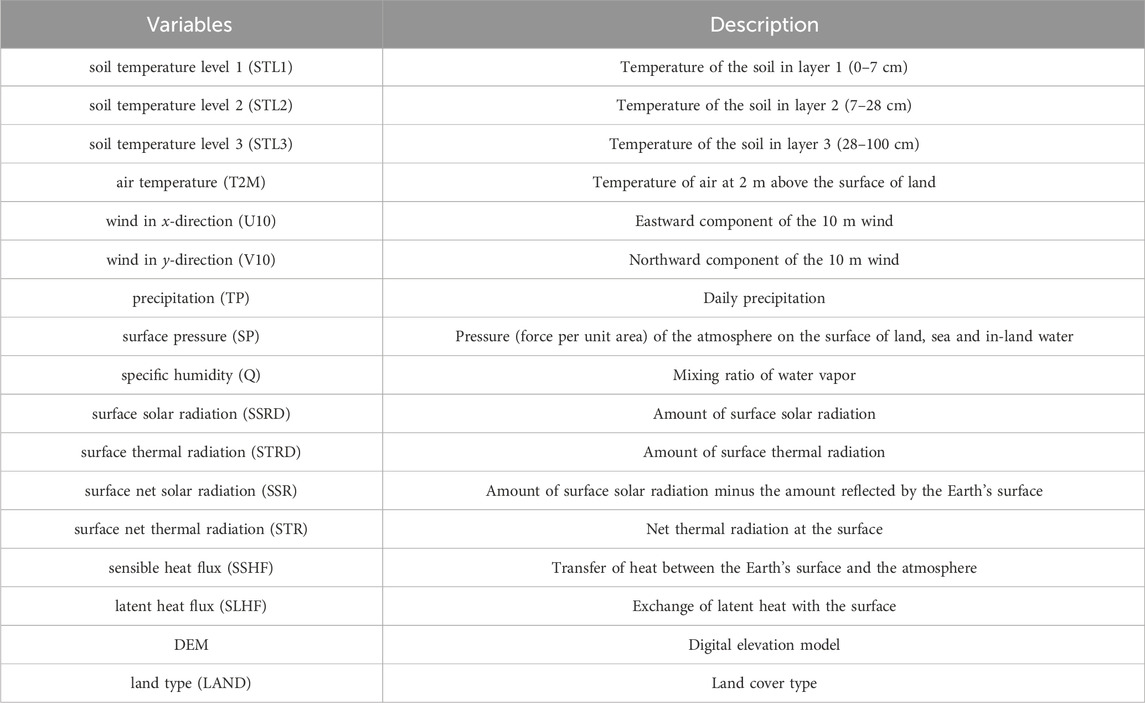
. Explanations and abbreviations of variables.