Landcover-categorized fires respond distinctly to precipitation anomalies in the South-Central United States

Satellite detection of active fires has contributed to advance our understanding of fire ecology, fire and climate dynamics, fire emissions, and how to better manage the use of fires as a tool. In this study, we use active fire data of 12 years (2012–2023) combined with landcover information in the South-Central United States to derive a monthly, open-access dataset of categorized fires. This is done by calculating a fire predominance index used to rank fire-prone landcovers, which are then grouped into four main landscapes: grassland, forest, wildland, and crop fires. County-level aggregated analyses reveal spatial distributions, climatologies, and peak fire months that are particular to each fire type. Using the Standardized Precipitation Index (SPI), it was found that during the climatological fire peak-month, the SPI and fires exhibit an inverse relationship in forests and crops, whereas grassland and wildland fires show less consistent inverse or even direct relationship with the SPI. This varied behavior is discussed in the context of landscapes’ responses to anomalies in precipitation and fire management practices, such as prescribed fires and crop residue burning. In a case study of Osage County (OK), we find that large wildfires, known to be closely related to climate anomalies, occur where forest fires are located in the county and absent in areas of grassland fires. Weaker grassland fire response to precipitation anomalies can be attributed to the use of prescribed burning, which is normally planned under environmental conditions that facilitate control and thus avoided during droughts. Crop fires, on the other hand, are set to efficiently burn residue and are practiced more intensely in drier years than in wetter years, explaining the consistently strong inverse correlation between fires and precipitation anomalies. In our increasingly volatile climate, understanding how fires, vegetation, and precipitation interact has become imperative to prevent hazardous fire conflagrations and to better manage ecosystems.

1 Introduction

The climatology of biomass burning in the United States points to the South-Central United States as one of the locations with the highest fire density in the country, especially in spring and fall (Lin et al., 2014; Kaulfus et al., 2017). In this region, fires are varied in nature. They can be prescribed to manage ecosystems (White and Hanselka, 1994; Ford and Grace, 1998; Baker et al., 2019; Kupfer et al., 2020; Bidwell et al., 2021), be used to burn crop residue following harvest (McCarty et al., 2007; Korontzi et al., 2008; McCarty, 2011; Pouliot et al., 2017), and occur unintentionally as wildfires (Reid et al., 2010; Barbero et al., 2015; Nagy et al., 2018; Burke et al., 2021). The type of fires on the ground can be identified by direct observation, which might be limited by the spatial range that a group of observers can cover. Conversely, satellite-based remote sensing provides global coverage of active fires in the form of points of high surface temperature (fires). One such product is the Moderate Resolution Imaging Spectroradiometer (MODIS), which provides daily active fire data points since March 2000 (to current) at 1 km spatial resolution (Justice et al., 2002). Similarly, the Visible Infrared Imaging Radiometer Suite (VIIRS) (Schroeder and Giglio, 2017b) provides global information of active fires beginning in January 2012 (to current) at a more refined spatial resolution (375 m) than MODIS. Among the advantages of using remote sensors is the availability of information in locations where in situ fire monitoring is scarce or absent, and the consistent methodology over an extended period of time, which facilitates studies of climate and fires relationships (Lin et al., 2014; Fernandes et al., 2017; Nogueira et al., 2017; Abatzoglou et al., 2018; Kumari and Pandey, 2020).

However, remote sensors do not discern what is burning on the ground during active fires. One strategy to overcome this limitation is to pair active fire data with landcover information to determine, at the pixel or administrative boundary levels, the landscape overlapping the satellite-detected fire. This can be done by evaluating fires in one landcover of interest (McCarty et al., 2007; Baker et al., 2019; McGranahan and Wonkka, 2024) or various landcovers in a particular area of study (Wiedinmyer et al., 2006; Gutiérrez-Vélez et al., 2014; Saim and Aly, 2022). Datasets that provide information of fires discriminated by landcover exist for Brazil, yearly, since 1985 (Alencar et al., 2022) and daily for four landcover types of the Amazon biome (Andela et al., 2022). Classifying fires according to landcovers has numerous applications, which include estimating carbon (Wiedinmyer et al., 2006; Sleeter et al., 2018; Ramo et al., 2021; Zheng et al., 2021) and particulate matter emissions from fires (McCarty, 2011; Pouliot et al., 2017; Baker et al., 2019; Maffia et al., 2020), managing ecosystems fires (Nyman and Chabreck, 1995; Knapp et al., 2009; Bidwell et al., 2021; Wilcox et al., 2022; Jaime et al., 2023), and advancing studies at the intersection of human activities, climate, and fires (Uriarte et al., 2012; Lin et al., 2014; Kupfer et al., 2020; Burke et al., 2021; Fernandes et al., 2022).

With that in mind, we developed a method to produce a monthly dataset of fires classified by the predominant landscape. Then, we use the dataset to address the question of whether fires respond differently to precipitation anomalies according to the landscape they occur in. The steps to accomplish that consist of combining 12 years (2012–2023) of high spatial resolution (375 m) VIIRS active fires (Schroeder and Giglio, 2017b) with the United States Department of Agriculture Cropland Data Layer (CDL) annual product (Boryan et al., 2011) to derive a fire predominance index in the south-central region of the United States. Then, the fire predominance index is ranked, and the top 10 landcovers with the highest fire incidence are combined into four groups, namely, grassland, forest, wildland, and crop fires. This reproducible numerical method and the resulting classification facilitate the climate and fire relationship analyses in distinct landscape groups. Last, fire sensitivity to variations of the Standardized Precipitation Index (McKee et al., 1993) is evaluated for each group’s climatological peak fire month and discussed in the context of fires’ response to climate stress, and fire use and management. We complement our analyses with a case study for the Osage County in Oklahoma, where fires of two categories, grasslands and forests, are common and relate distinctively to precipitation anomalies.

2 Materials and methods

2.1 Study area

The focus area of our study comprises the south-central sector of the United States, which is bounded by the coordinates 100^oW–87^oW and 29^oN–42^oN. We chose the domain of study to include an area of high fire activity (Kaulfus et al., 2017; Hawbaker et al., 2020), varied landcovers (Supplementary Figure S2), and annual precipitation amounts driven by climate patterns characteristic of the eastern side of the Rocky Mountains (Supplementary Figure S1).

2.2 Data

2.2.1 VIIRS fires

Fire detection from the Visible Infrared Imaging Radiometer Suite (VIIRS) instrument onboard of the Suomi National Polar-orbiting Partnership (S-NPP) satellite is used in our study. The daily VIIRS product at a resolution of 375 m pixel (VNP14IMG) consists of a fire mask, in which three classes identify low, nominal, and high confidence levels of active fire detection (Schroeder and Giglio, 2017b). The VIIRS dataset, publicly available from NASA FIRMS (https://firms.modaps.eosdis.nasa.gov/), is obtained as a table in which the latitudinal and longitudinal coordinates of a detected fire is provided daily. The coordinates of an active fire represent the center of the VIIRS pixel and are used to rasterize the point data into a 375-m resolution grid over the entire domain of study. The daily VIIRS raster file is then added to monthly totals from February 2012 to December 2023.

2.2.2 Cropland data layer (CDL)

The Cropland Data Layer (CDL) provides a geo-referenced, 30-m spatial resolution crop and other landcover classifications for the United States (Han et al., 2012). The CDL is updated annually since 1997 and contains 90 classes for different types of crops, natural landscapes, and various levels of urban development. We use the CDL resource in combination with the VIIRS active fires data to derive an index describing which landscapes are most susceptible to fires within our study area.

2.2.3 Standardized Precipitation Index—gridMET

The Gridded Surface Meteorological (gridMET) dataset is a daily surface meteorological dataset covering the contiguous US (Abatzoglou, 2013). It combines the PRISM gridded climate data (Daly et al., 1994) and the regional reanalysis NLDAS-2 (Mitchell et al., 2004) to produce a spatially and temporally complete 4-km gridded dataset beginning in 1979 and updated daily to current dates. The daily precipitation from gridMET is first aggregated to monthly totals and then the 1-month Standardized Precipitation Index (SPI) is calculated (McKee et al., 1993). The SPI is the number of standard deviations that the observed cumulative precipitation deviates from climatology and can be used to assess equally positive and negative anomalies, requiring only precipitation for its calculation.

2.3 Methods

2.3.1 Landcover re-classification

Given the difference in spatial resolution between the CDL and VIIRS active fires, we first calculate a histogram of the 30-m resolution CDL classes within each VIIRS 375-m pixel. Then, we retain only pixels in which one single CDL class covers at least 70% of the VIIRS pixel area and make the assumption that if a fire was registered within the said pixel, the most likely landscape burned is the one covering 70% or more of the pixel area. This is done for every year between 2012 and 2023, and the output raster consists of a CDL 375-m classification containing only pixels in which there was a single class majority (Supplementary Figure S2). Our objective is to evaluate vegetation fires; thus, we excluded classes that describe development and water, as well as the CDL class “not defined.”

2.3.2 Fire predominance per landcover class

To calculate a fire predominance index per landcover class, an annual VIIRS layer that consists of a mask identifying any number of fires within the year as “1” and no-fire as “0” is created. The pixels marked as “1” are combined with the reclassified landcovers to produce a spatial predominance of fire occurrence according to the landcover. In other words, when the VIIRS mask layer is multiplied by the reclassified CDL layer, only classes in which fires occurred (CDL class multiplied by 1) are retained. Then, the “landcover-classified fires” are counted annually (number of pixels with at least one fire in class, NPx_(1FC), in Eq. 2) over the 2012–2023 period.

Simply ranking the CDL classes in which fires occurred, as described above, may be misleading due to the relative prevalence of a certain landcover class. For instance, more fires may be observed in a certain landcover (e.g., corn compared to watermelon) just because that landcover class occurs more often in our domain. Thus, instead of a simple count of fire pixels by class, we calculate a fire spatial predominance (FSP_C in Eq. 2) as the number of fire pixels in a class (NPx_(1FC)) divided by the total number of pixels in that class (TNPxC in Eqs 2, 3) within the domain of study. Thus, the total number of fire pixels classified as occurring in corn fields (for example) is divided by the total number of pixels (at the 375-m resolution) classified as corn. This provides a relative metric that accounts for how many “corn-fire pixels” were detected in a year in relation to the predominance of the corn area.

One final weighting is necessary to reduce the influence of fires in landcovers that are uncommon in the area of study. For example, if one single fire is classified as occurring in a watermelon pixel and the total number of pixels classified as watermelon is four, the above adjustment would point to a 25% predominance of fires in watermelon fields, which would suggest that every fourth watermelon pixel will experience a fire in a given year. However, this high incidence rate is more likely due to the instability of rate calculations with small sample sizes, and fires in such an uncommon landcover are not the focus of this study. Another adjustment is therefore applied, in which the fire spatial predominance in a class (FSP_C) is multiplied by the overall prevalence of that landcover class in the domain of study (CP_Domain). CP_Domain (Eq. 3) is calculated as the total number of pixels in a class (TNPxC) divided by the total number of pixels in all classes (TNPx in Eq. 3) that registered fires (excluding “not-defined” CDL classes). The final metric resulting from these calculations becomes a fire predominance index (FPI in Eq. 1), which is used to describe the landcovers with the highest fire occurrence over the 12 years of VIIRS data. In our initial approach, we adjusted FPI for multiple fires in one pixel by multiplying it by the ratio between the annual total number of fires in a class and NPx_(1FC). The ratio resulted mostly in values of 1 (only one fire detected in a pixel) and an occasional value of 1.3, indicating that in some years, up to 30% of pixels will report multiple fires in specific landcovers. The resulting FPI ranking was not different from that reported in Section 2.3.3, and we chose to eliminate this step for simplicity.

$\text{FPI}={\text{FSP}}_{\mathrm{C}}\mathrm{X}{\text{CP}}_{\text{Domain}},(1)$

${\text{FSP}}_{\mathrm{C}}=\left({\text{NPx}}_{\left(1\text{FC}\right)}/\text{TNPxC}\right)*100,(2)$

${\text{CP}}_{\text{Domain}}=\left(\text{TNPxC}/\text{TNPx}\right)*100,(3)$

where FPI is the fire predominance index, FSP_C is the fire spatial predominance, NPx_(1FC) is the number of pixels with at least one fire in class, TNPxC is the total number of pixels in class, CP_Domain is the class predominance in the domain of study, and TNPx is the total number of pixels in all classes that registered fires. The 100 factor is introduced for scaling purposes only.

2.3.3 Fire predominance groups

The fire predominance index above is averaged among the 2012–2023 period and ranked to determine the landcovers with the highest fire occurrence. The ranking highlights 10 main landcovers in terms of fire occurrence that are then grouped into categories, namely, “grassland,” “forest,” “wildland,” and “crop” (Table 1). The category “wildland” groups fires that occur in native landcovers other than grasslands and forests. Once the groups are determined, the original annual CDL landcover layer (at 30-m resolution) is processed to eliminate the landcovers that were not significant concerning fire predominance (classes not in Table 1) or were of a non-vegetation category such as developed (cities), water, and not-defined classification. Then, the classes identified by the fire predominance index are assigned a group number. Grassland becomes “1,” forest “2,” wildland “3,” and crop “4.”

Table 1

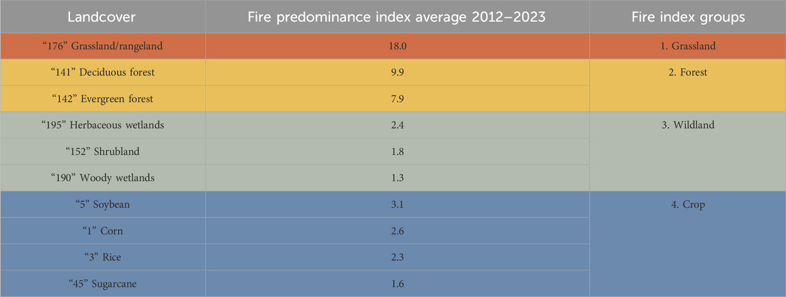
Table 1. Fire predominance according to landscape.

By replacing the 30-m resolution CDL layer with the fire predominance index groups, we reduce the landcovers to retain only those we identify as most fire prone in our domain of study. Then, the CDL layer with reduced classes is again processed to result in a histogram to determine the predominant group within the 375-m VIIRS pixel. The pixels in which a single fire group class (among the four described in Table 1) covers at least 50% of the pixel area are retained, and the predominant group class is recorded. Pixels where there is no clear majority among the four defined classes are coded as no data. The reason for retaining pixels with a clear single majority is to reduce misclassification, as we assume that an active fire that overlays a pixel classified as 50% forest (for example) is more likely than not to have occurred over a forest. This approach is likely to result in some misclassification, but a 100% exact classification is also limited by the fact that the VIIRS product provides the geographical coordinates of an active fire (a point), and those coordinates correspond to the center of a pixel of 375-m by 375-m, but the actual fire could have occurred anywhere within that pixel area. Another caveat of the reduced classification is that some active fires detected by VIIRS will overlap with vegetation classes that were not identified by our method as the most fire prone. We calculated, annually, the percentage of VIIRS active fires that overlap vegetation pixels other than those in Table 1 and determined that between 9% and 13% of active fires in any given year are not accounted for. The final classification of fire predominance groups is shown in Supplementary Figure S3 for 2022, and the methodology workflow is shown in Figure 1.

Figure 1

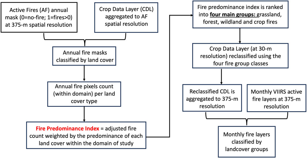
Figure 1. Workflow of the methodology to obtain the fire predominance index, landcover fire groups, and monthly fire typology layers.

The final step combines each year’s CDL classification identifying the four main fire groups (Supplementary Figure S3) with same year monthly VIIRS active fires to produce a dataset consisting of four layers per month. For example, for December 2023, a raster layer with pixel fire count was available for grassland, forest, wildland, and crop separately. By providing separate layers, users can take advantage of evaluating only the type of fire of interest and obtain the total monthly fire count (for each type) detected by VIIRS at the pixel level. Alternatively, users can combine the layers to obtain monthly (or derived time aggregates) fire counts for the four types of fires. An example for the entire year of 2022 (Figure 2) in southern Louisiana shows an area of forest fires to the north, crop fires to the east along the Mississippi River Delta, and wildland fires to the south along the coastal wetlands.

Figure 2

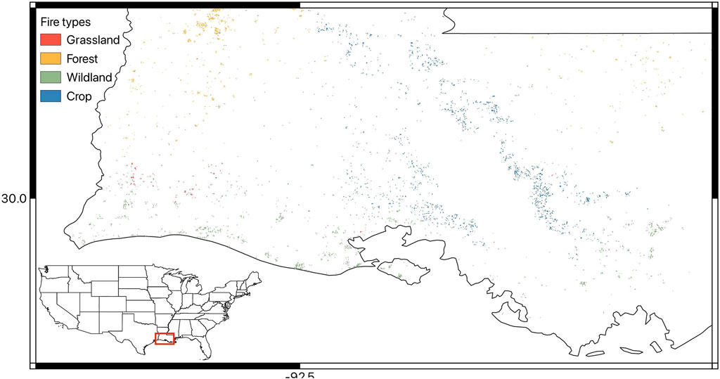
Figure 2. VIIRS active fires classified by type in southern Louisiana in 2022. The shades represent the type of fire as per our fire predominance index at pixels with any number of fires within the year. The southern Louisiana sector zoomed in is marked with a red box in the United States map.

2.3.4 Fire and climate characterization at the county level

We evaluate the climatological characteristics and spatial distribution of fires by aggregating the fire count to the county administrative level for each type of fire and all 975 counties in the domain of study. For example, if in a county there are 10 pixels identified as forest fires and each had 2 fires in January 2022, those data will be stored as January 2022 = 20 forest fires. If that same county had another 10 pixels with one grassland fire each in January 2022, then those data will be stored separately as January 2022 = 10 grassland fires. From the time series, we calculate the monthly climatology for each type of fire and determine the month with the highest (peak) climatological count for each type separately. Then, for each fire type, the 10% (98 counties—Supplementary Table S1) counties with the highest fire count during their respective peak-month are retained and correlated with the peak-month SPI. The peak-month SPI is averaged over pixels that overlap the fire type of interest. We are also interested in comparing correlations between each type of fire and the SPI with correlations between all-fires and the SPI. To do that, all VIIRS active fire pixels are counted within a county, then the climatological peak month is defined, and correlations with the peak-month SPI (averaged over the entire county domain) are performed. Correlation significance is described as p-value performed with a two-tailed t-test and reported as non-significant for P-value greater than 0.1.

3 Results

3.1 Grassland fires

The counties with the highest incidence of grassland fires are located mainly in central-eastern Oklahoma and Kansas, where the peak activity months are March and April. The average all-fires count (Figure 3A) during the peak month is very similar to that of grassland (Figure 3B), indicating that this is the main type of fire occurring in most of the displayed counties. There are a few counties where the all-fires count is clearly higher than the grassland fires count, Osage County in Oklahoma (darkest shade in Figure 3A) being one that stands out with an average all-fires count of 1,015 and grassland fires count of 606 during the climatological peak (month of April). We will discuss the results of Osage County in more detail in Section 3.5.

Figure 3

Figure 3. Climatological (2012–2023) peak-month fire count for VIIRS (A) all-fires and (B) grassland fires. Peak month, defined as the month with the highest climatological fire count, is shown as a number at the center of the county.

When evaluating fires and climate, a general synchronous inverse relationship between fires and precipitation is expected (Reid et al., 2010; Morton et al., 2013; Saim and Aly, 2022). However, human-related activities such as fire ignition and management can make this relationship less straightforward (Hawbaker et al., 2013; Baker et al., 2019; McGranahan and Wonkka, 2024). In counties where grassland fires are most prominent, correlations between all-fires and the peak-month SPI (Figure 4A) show clusters with both direct and inverse relationships between the variables. In eastern Kansas, fires and the peak-month SPI are positively correlated, and in southern Oklahoma and southeastern Kansas, all-fires and the SPI are negatively correlated. Grassland fires (Figure 4B) and SPI correlations show a similar pattern, suggesting that all-fires and SPI relationships generally represent those of grassland fires and the SPI. In southern Oklahoma, grassland fires and SPI correlations tend to be weaker than all-fire and SPI correlations, suggesting that other types of fires are observed during the peak month. In this region, some of the counties in which grassland fires are common are also among the counties in which forest fires also occur.

Figure 4

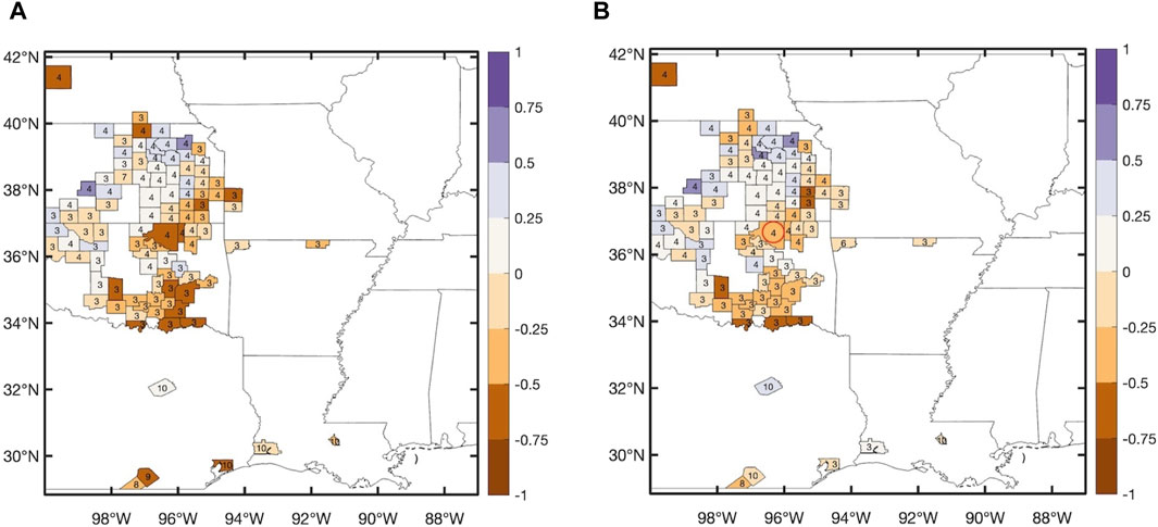
Figure 4. Correlation between peak-month VIIRS (A) all-fires and (B) grassland fires with 1-month SPI. Peak-month SPI is averaged over the counties’ entire domain for the correlations in (A) and averaged over pixels that overlap grassland fires for correlations in (B). Correlation values greater than absolute 0.5 are statistically significant (P < 0.1, two-tailed t-test). The counties shown represent the 10% with the highest grassland fire count during the peak month. Osage County (OK) is marked with a red circle.

3.2 Forest fires

Similar to grassland fires, forest fires’ peak activity months are concentrated in early spring. The counties with the highest incidence extend from eastern Oklahoma to central Arkansas and southern Missouri. Some other clusters are found in Louisiana, Texas, Mississippi, and Alabama. In eastern Oklahoma, some of the counties that are among the top 10% for forest fires incidence (Figure 5B) are also among the top 10% highest grassland fires (Figure 3B). The all-fires climatological count (Figure 5A) is very similar to the forest fires peak-month count, except in eastern Kansas and northern Oklahoma, whereas in some counties, the all-fires count includes forest (Figure 5B) and grassland (Figure 3B) fires. The all-fires peak months coincide with the forest peak months, except for a couple of parishes in western Louisiana, indicating that forest fires are not the main driver of the high fire count.

Figure 5

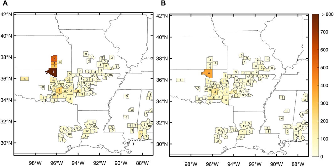
Figure 5. Climatological (2012–2023) peak-month fire count for VIIRS (A) all-fires and (B) forest fires. Peak month, defined as the month with the highest climatological fire count, is shown as a number at the center of the county.

All-fires and peak-month SPI correlation (Figure 6A) shows a predominance of negative correlation values, which generally become more widespread and more robust for forest-only fires and the SPI (Figure 6B). This behavior is distinct to that observed between grassland fires and the SPI, suggesting that in counties where forest fires predominate, the response to precipitation anomalies are more direct and possibly more closely related to wildfires than to controlled burns that are typical of grasslands in our domain. We will discuss this argument further in Section 3.5.

Figure 6

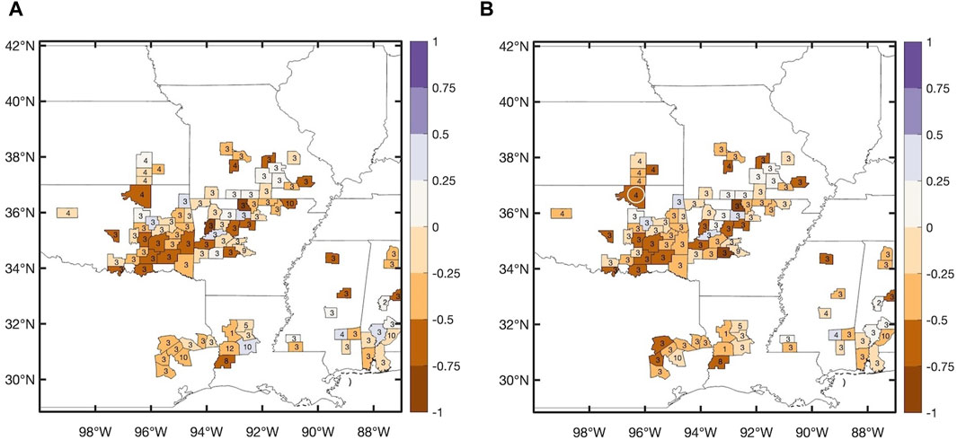
Figure 6. Correlation between peak-month VIIRS (A) all-fires and (B) forest fires with 1-month SPI. One-month SPI is averaged over the counties’ entire domain for the correlations in (A) and averaged over pixels that overlap forest fires for correlations in (B). Correlation values greater than absolute 0.5 are statistically significant (P < 0.1, two-tailed t-test). The counties shown represent the 10% with the highest forest fire count during the peak month. Osage County (OK) is marked with a white circle.

3.3 Wildland fires

As per our fire predominance index, wetlands and shrublands (Table 1) are among the landcovers with high fire frequency. Even though wetlands and shrublands are normally found in different climate regimes (wet and dry), the spatial distribution of our reduced classification would allow for an identification of the main landcover according to its location. Thus, we group these landcovers in one category and call “wildland” fires to classify fires in native vegetation that are not grasslands or forests.

The distribution of the counties with the 10% highest fire count in this category highlights the wetlands along the Gulf of Mexico and shrubland in central Texas. Other clusters are located along the Mississippi River plains and central-western Louisiana (Figure 7B). By evaluating the all-fires count during the climatological peak-month (Figure 7A), we can visually determine that wildland fires co-occur with other types of fires in some areas. For example, the all-fires count in Mississippi County, Arkansas (darkest shaded county in Figure 7A), shows an average of 311 fires during its climatological peak (month of September), but only a fraction of it is wildland fires, suggesting other types of fires dominate the fire regime in this location.

Figure 7

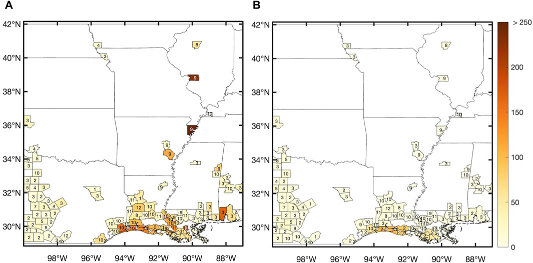
Figure 7. Climatological (2012–2023) peak-month fire count for VIIRS (A) all-fires and (B) Wildland fires. Peak month, defined as the month with the highest climatological fire count, is shown as a number at the center of the county.

Although it may seem counterintuitive to observe fires in wetlands, they are in fact common due to the seasonality of precipitation regimes with distinct dry periods, anthropogenic interventions (dams, canals, and levees) that change the natural flooding cycle of rivers, and climate change that impacts sea level rise and, consequently, ecosystems, health, and/or precipitation regimes of wetlands (Williams-Jara et al., 2022). Wetland fires tend to be inversely correlated with the peak-month SPI, as seen along the Gulf of Mexico coast and interior Louisiana (Figure 8B). A weaker coupling between all-fires and the SPI (Figure 8A) is observed in some of the counties in this sector, suggesting that fires in a landcover other than wetlands are also contributing to the general fire response to precipitation anomalies.

Figure 8

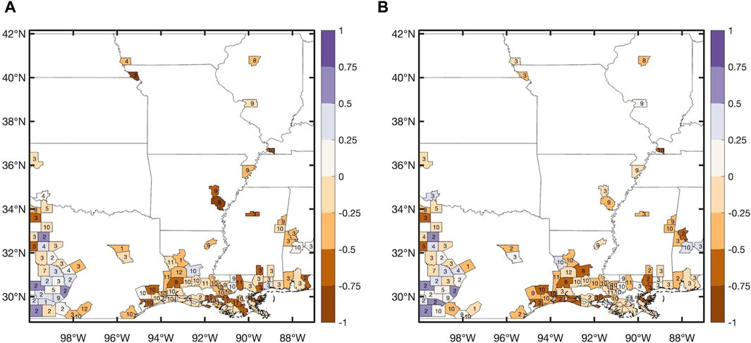
Figure 8. Correlation between peak-month VIIRS (A) all fires and (B) wildland fires with 1-month SPI. One-month SPI is averaged over the counties’ entire domain for the correlations in (A) and averaged over pixels that overlap wildland fires for correlations in (B). Correlation values greater than absolute 0.5 are statistically significant (P < 0.1, two-tailed t-test). The counties shown represent the 10% with the highest wildland fire count during climatological peak month.

3.4 Crop fires

Fires are used as an inexpensive and labor-saving method to burn crop residue following harvesting, as a form of pest control, and to clear land for planting. The practice is commonly used in the Southeastern US (McCarty et al., 2007; McCarty, 2011; Lin et al., 2014), especially along the Mississippi River Alluvial Plain from southeastern Missouri to Louisiana (Korontzi et al., 2008), and most of the top 10% fire count counties in the crop category are found along this region (Figure 9). The main crops identified with high fire predominance are rice, corn, and soybeans mainly in Arkansas and sugarcane in Louisiana. Consistent with the timing of the main harvest in the southeast, crop fires occur mainly in September and October in the counties among the 10% with highest crop fire count (Figure 9B). The all-fire climatology (Figure 9A) reveals a very similar picture of timing (peak month) and count, indicating that fires in these counties are dominated by crop fire regimes.

Figure 9

Figure 9. Climatological (2012–2023) peak-month fire count for VIIRS (A) all-fires and (B) crop fires. Peak month, defined as the month with the highest climatological fire count, is shown as a number at the center of the county.

Among the four fire types, fires in crops show the most robust and inverse relationship with the SPI across the various counties. The all-fire correlation with the SPI is very similar to correlations calculated for crop fires only and the SPI, indicating that in the majority of counties shown in Figure 10, the climate–fire relationship is dominated by the sensitivity of crop fires to precipitation anomalies during the peak month.

Figure 10

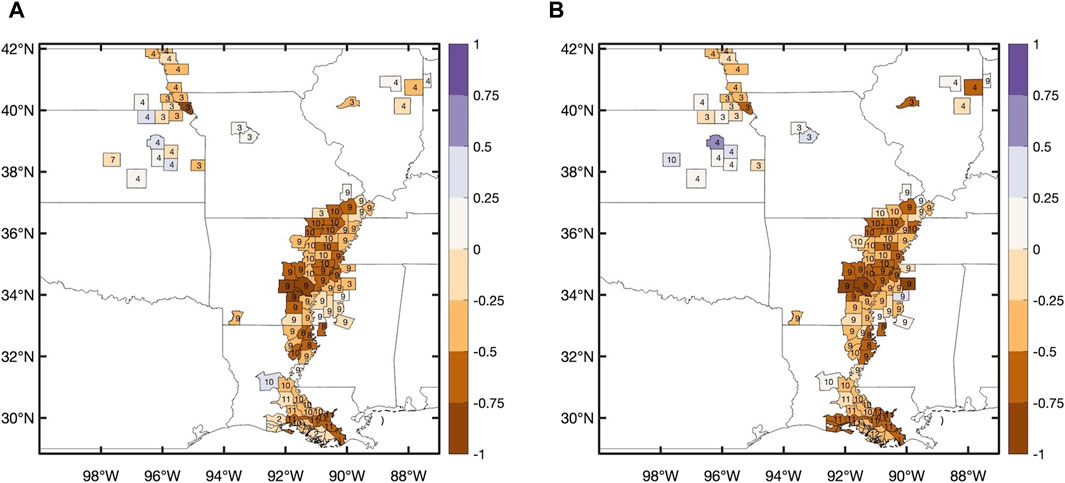
Figure 10. Correlation between peak-month (A) VIIRS all-fires and (B) crop fires and peak-month SPI. SPI is averaged over the counties’ entire domain for the correlations in (A) and averaged over pixels that overlap wildland fires for correlations in (B). Correlation values greater than absolute 0.5 are statistically significant (P < 0.1, two-tailed t-test). The counties shown represent the 10% with the highest wildland fire count during climatological peak month, shown at the center of the county.

3.5 Case study: Osage County, OK

The county with the highest all-fire climatological fire count in our domain of study is Osage County in Oklahoma, where grassland and forest fire types predominate (Figures 3, 5) with the peak month in April. Active fires in spring are consistent with the practice of prescribed burns being carried out when high moisture content in new vegetation makes it easier to control the burning (Weir et al., 2009). Prescribed fires in Oklahoma are used every year with the goal of controlling invasive woody species, conserve and/or restore native ecosystems, and reduce the risk of large wildfires in overgrown prairies and forests (Bidwell et al., 2021). Spring is also the season with a high risk of wildfires caused by lighting and greater (or lower) potential for uncontrolled spread according to precipitation anomalies during the life of a wildfire event (Weir et al., 2009; Reid et al., 2010). Thus, we chose Osage County for a case study to illustrate the potential for evaluating fires according to landcover, given the varied nature of fires in the county. Grassland fires occur almost twice as much as forest fires; thus, we standardize the fire count (subtract each fire type climatology and divide by standard deviation) to depict a time series of April grassland and forest fire anomalies in Osage County (Figure 11).

Figure 11

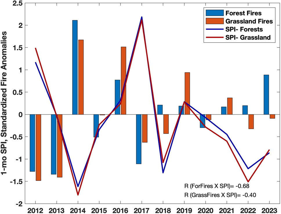
Figure 11. Osage County (OK) April standardized fire anomalies (bars) in grassland and forests. The lines represent April 1-month SPI for each type of fire obtained by averaging SPI over pixels that overlap forest and grassland fires. The correlations (R) between fires and SPI for both forest and grassland are shown at the bottom.

The correlation between April (2012–2023) all-fires and the county-averaged April 1-month SPI is negative (R = −0.55, P < 0.06, two-tailed t-test), as expected in a response of more fires associated with deficient precipitation (Figures 4A, 6A). Figure 11 shows the time series of April standardized grassland and forest fire anomalies along with the SPI averaged over pixels corresponding to each type of fire within Osage County. The time series shows more clearly the correlations shaded in Figures 4B, 6B, where Osage County is marked with a circle. April grassland fires and the SPI correlate negatively, but the strength of this relationship is weaker (R = −0.4, P < 0.2, two-tailed t-test) than that obtained from all-fires and the SPI. For instance, April of 2018, 2022, and 2023 were dry in Osage County and yet, grassland fires show an anomalously low count. This weaker grassland fires response to droughts is likely related to the use of prescribed fires, which is carried out in a wetter environment, weakening or possibly reversing the typical negative correlation between drought and fires. It is also important to recognize that vegetation may respond to climate conditions with a time lag (Littell et al., 2009; Morton et al., 2013; Barbero et al., 2015), which is an effect that is not explored here. Other studies attribute the poor precipitation and fires relationship to fire–grazing interactions, as in dry conditions, grazed areas will take longer to recover, leading to a reduced fuel load (Bekker and Taylor, 2001; McGranahan and Wonkka, 2024) and reduced fire occurrence, regardless of the climate.

Conversely, forest fires and SPI correlation is the strongest (R = −0.68, P < 0.01, two-tailed t-test) among the three. This behavior can be seen in Figure 11, as the negative SPI (dry) tends to be more consistently related to positive anomalies in forest fires (2014, 2018, 2021, 2022, and 2023) and neutral (−0.3< SPI <0.3) to the positive SPI are related to less forest fires (2012, 2013, 2015, 2017, and 2020). Our results are consistent with those of Lin et al. (2014), who used potential evaporation (PE) as a metric of atmospheric dryness (high PE = dry; low PE = wet). The authors found a weak negative correlation between prescribed fires and PE and a more robust positive correlation between large wildfires and PE in northern Oklahoma. Larger wildfires have been found to show a more robust response to precipitation anomalies (Reid et al., 2010; Barbero et al., 2015; Nagy et al., 2018), and we checked whether the more robust correlation between forest fires and precipitation is related to the nature and size of fires in the county. To accomplish that, we overlaid the Monitoring Trends in Burn Severity (Eidenshink et al., 2007) (MTBS) burned area for wildfires greater than 500 acres with the total grassland and forest fire counts for April (2012–2023). The burned areas obtained from MTBS correspond to wildfires with ignition in the last week of March or in April from 2012 to 2023. The reasoning for retaining burned areas with ignition in the last week of March is that a large wildfire will likely burn for a few days, thus persisting into April. Most large wildfires indeed occurred in the eastern sector of the county, where forest fires pixels (blue shades in Figure 12) either predominate or are mixed with grassland fires. In other words, conflagrations that occur in areas of forests in Osage County are more likely to become large in a more direct response to droughts, in contrast to grassland fires that show a weaker response to precipitation anomalies.

Figure 12

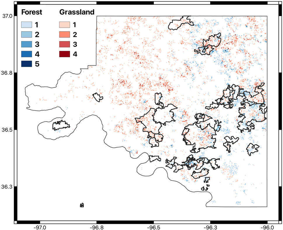
Figure 12. Total fire count for the month of April (2012–2023) in Osage County, OK. The red shades represent pixels classified as grassland fires and blue shades represent pixels classified as forest fires. The contour areas mark the burned areas of large wildfires (>500 acres) that occurred between 2012 and 2023 during the month of April.

4 Discussion

When evaluating the effects of climate on vegetation fires, one important ally comes in the form of remote sensing fire detection, assessed as thermal anomalies at the surface (Justice et al., 2002; Schroeder and Giglio, 2017a). In our study, we combined active fires from the VIIRS sensor with landcover to determine four main fire type groups in the south-central United States: “grassland,” “forest,” “wildland,” and “crop” fires. Other studies have evaluated active fires according to landcovers but at coarser spatial resolution and with pre-determined classes of interest (McCarty et al., 2007; Lin et al., 2014), whereas our method objectively ranks the landcovers where fires predominate at a spatial resolution of 375-m. The main motivation to produce this fire typology dataset was to answer the question of whether fires occurring in varied landscapes demonstrate different sensitivity to precipitation anomalies assessed by the Standardized Precipitation Index. The fire typology dataset was then processed to provide the climatological characteristics of each of the four types and an analysis of SPI and fires correlations aggregated to the county administrative levels.

We report our main results for the counties that were among the 10% (98) with the highest fire count during the climatological peak month for each type of fire (Supplementary Table S1). Fires in grasslands become a category on their own, as they emerged as the landcover with the highest fire incidence in our area of study. The top 10% grassland fire count counties show the fire peak month in spring in a cluster distributed over Kansas and Oklahoma. Correlations of peak-month grassland fires and the SPI show a statistically non-significant positive relationship in a large sector of Kansas. This is consistent with grassland/rangeland fire management in the Flint Hills region, where prescribed fires are set under environmental conditions that minimize the risk of uncontrolled spread, leading to a partial decoupling between droughts and fires (Baker et al., 2019). Areas of negative correlation, although mostly statistically non-significant, are observed in Oklahoma, where grasslands are found in mosaics with other types of vegetation such as crops and forests. This becomes evident from our case study in Osage County in Oklahoma, where grassland fires are more weakly coupled to precipitation anomalies than forest fires, likely due to the greater accumulation of dry fuel in forests and greater susceptibility to climate (Littell et al., 2016).

The third ranked group of fires derived from our index was labeled wildland fires, and it represents two main types of landcovers: wetlands and shrublands. In the wetlands of Louisiana, the main fire season is fall, and correlations with the SPI, mostly statistically significant, follow the expected inverse relationship of more fires during dry years. In the shrublands of Texas, the main fire season is late winter and spring, and SPI and fire correlations during the peak fire month describe a weak coupling. This behavior is similar to that reported in grasslands, where the use of prescribed fires in the eastern sector of the Edwards Plateau and the Rolling Plains helps manage the encroaching of woody species, such as shrubs and trees, into the natural grassland ecosystem of the region (Brown and Smith, 2000; Wilcox et al., 2022; Jaime et al., 2023). The less than straightforward relationship between fires and climate results from prescribed burns being carefully set to prevent unintended spread, leading to a decoupling with droughts (Barbero et al., 2015; Nowell et al., 2018).

Crop fires represent the fourth type derived from our methodology. The 10% counties with the highest fire count during the peak month align along the Mississippi River Alluvial Plain extending from Arkansas to Louisiana. The peak crop fire season is fall, which is consistent with the practice of crop residue burning following harvest. Wildland fires are also frequent in some coastal Louisiana counties where crop fires are common, but the peak fire month occurs instead in late winter. Of all four groups, inverse and statistically significant correlation is observed most consistently between the SPI and crop fires. In contrast to prescribed burnings in native vegetation that are avoided in years of drought (Baker et al., 2019), our results suggest that crop fires are managed to take advantage of dryer conditions, as the main objective is to optimize the task and reduce costs, leading farmers to burn more in dry years and less in wet years (Lovett, 2022).

Our approach is not free from limitations: the non-inclusion of vegetated landcovers that registered fires but were not among the classes we ranked as the most relevant in our domain. In addition, a fire pixel is classified if a minimum of 50% of the area within the said pixel is covered by one of the four groups identified in our ranked index. Thus, at any given year, there is between 9% and 13% of fire pixels that remain unclassified and are not included in our analyses.

Last, the results presented in this study illustrate only one example of various analyses that can be conducted with an active fire dataset classified by landcover types. Some other applications include modeling the effects of socioeconomic variables on different types of fires, combining the fire typology dataset with prescribed and wildfire data to better understand the effectiveness of fires used as a natural disaster prevention and ecosystem management tool in different landscapes, determining the relationship of fire types to climate variables beyond that discussed in this study and other timescales of interest, and estimating fire emissions (particulate matter and carbon), as they are dependent on the type of vegetation burned. In addition, our straightforward methodology can be replicated in other sectors of the United States to rank the main types of landcovers in which fires, due to either natural processes or fire practices, occur. Our approach adds a layer of comprehension regarding the fire–climate–human intersection that is becoming increasingly necessary for hazardous fire prevention and management under current and future climate variability and change.

5 Conclusion

Satellite-based fire estimates provide essential information for fire and climate studies, especially in areas where other types of fire records are insufficient. By combining satellite-based active fires with landcover layers, we derived a dataset that provides monthly fire estimates identified by one of the four main groups, namely, grassland, forest, wildland, and crop fires, in the south-central sector of the United States. Not all active fire pixels are matched with one of the four types defined here, given the mismatch between the spatial resolution of the CDLs (30-m) and the VIIRS fire pixel (375-m), resulting in 9%–13% of active fire pixels annually that are left unclassified. This could be overcome by pairing higher spatial resolution fire datasets, such as Landsat (30-m resolution) hotspots (Schroeder et al., 2016), with the CDL layers. Landsat fires, however, have the disadvantage of a short time series as the product is available since June 2022. As our primary objective was to evaluate year-to-year variability of landscape fires and the SPI, we traded-off higher spatial resolution in favor of a longer time series. In doing so, we were able to characterize the four groups of vegetation fires in terms of their seasonality and climatological values. We also show that fires and climate relationships are not always straightforward as they can be modulated by human activities carried out in each landscape. Our method, dataset, and approach can support further studies to advance our understanding of the current and future climate impacts on fires in particular landscapes, and how we can adapt our practices to mitigate the risk of uncontrolled fires and their potential negative impacts on ecosystems.

Data availability statement

The datasets presented in this study can be found in online repositories. The names of the repository/repositories and accession number(s) can be found below: https://zenodo.org/records/11200553.

Author contributions

KF: conceptualization, data curation, formal analysis, funding acquisition, investigation, methodology, project administration, resources, software, supervision, validation, visualization, writing–original draft, and writing–review and editing. SY: conceptualization, methodology, validation, and writing–review and editing.

Finanzierung

The author(s) declare that financial support was received for the research, authorship, and/or publication of this article. This research was partially supported by startup funds from the Department of Geosciences at the University of Arkansas.

Acknowledgments

Author KF acknowledges the support of the North Carolina State Climate Office. The authors thank Columbia University’s International Research Institute for Climate and Society (IRI) Climate Data Library for disseminating gridMET and facilitating data analyses. (https://iridl.ldeo.columbia.edu/SOURCES/.ClimatologyLab/.gridMET/.permanent/).

Conflict of interest

The authors declare that the research was conducted in the absence of any commercial or financial relationships that could be construed as a potential conflict of interest.

Publisher’s note

All claims expressed in this article are solely those of the authors and do not necessarily represent those of their affiliated organizations, or those of the publisher, the editors, and the reviewers. Any product that may be evaluated in this article, or claim that may be made by its manufacturer, is not guaranteed or endorsed by the publisher.

Supplementary material

The Supplementary Material for this article can be found online at: https://www.frontiersin.org/articles/10.3389/fenvs.2024.1433920/full#supplementary-material

References

Abatzoglou, J. T. (2013). Development of gridded surface meteorological data for ecological applications and modelling. Int. J. Climatol. 33, 121–131. doi:10.1002/joc.3413

CrossRef Full Text | Google Scholar

Abatzoglou, J. T., Williams, A. P., Boschetti, L., Zubkova, M., and Kolden, C. A. (2018). Global patterns of interannual climate–fire relationships. Glob. change Biol. 24, 5164–5175. doi:10.1111/gcb.14405

CrossRef Full Text | Google Scholar

Alencar, A. A., Arruda, V. L., Silva, W. V. da, Conciani, D. E., Costa, D. P., Crusco, N., et al. (2022). Long-term landsat-based monthly burned area dataset for the Brazilian biomes using deep learning. Remote Sens. 14, 2510. doi:10.3390/rs14112510

CrossRef Full Text | Google Scholar

Andela, N., Morton, D. C., Schroeder, W., Chen, Y., Brando, P. M., and Randerson, J. T. (2022). Tracking and classifying Amazon fire events in near real time. Sci. Adv. 8, eabd2713. doi:10.1126/sciadv.abd2713

PubMed Abstract | CrossRef Full Text | Google Scholar

Baker, K., Koplitz, S., Foley, K., Avey, L., and Hawkins, A. (2019). Characterizing grassland fire activity in the Flint Hills region and air quality using satellite and routine surface monitor data. Sci. total Environ. 659, 1555–1566. doi:10.1016/j.scitotenv.2018.12.427

PubMed Abstract | CrossRef Full Text | Google Scholar

Barbero, R., Abatzoglou, J. T., Kolden, C. A., Hegewisch, K. C., Larkin, N. K., and Podschwit, H. (2015). Multi-scalar influence of weather and climate on very large-fires in the Eastern United States. Int. J. Climatol. 35, 2180–2186. doi:10.1002/joc.4090

CrossRef Full Text | Google Scholar

Bekker, M. F., and Taylor, A. H. (2001). Gradient analysis of fire regimes in montane forests of the southern Cascade Range, Thousand Lakes Wilderness, California, USA. Plant Ecol. 155, 15–28. doi:10.1023/a:1013263212092

CrossRef Full Text | Google Scholar

Bidwell, T. G., Weir, J. R., Carlson, J., Masters, R. E., Fuhlendorf, S. D., Waymire, J., et al. (2021). Using prescribed fire in Oklahoma. Okla. Coop. Ext. ServAvailable at: https://extension.okstate.edu/fact-sheets/using-prescribed-fire-in-oklahoma.html.

Google Scholar

Boryan, C., Yang, Z., Mueller, R., and Craig, M. (2011). Monitoring US agriculture: the US department of agriculture, national agricultural statistics service, cropland data layer program. Geocarto Int. 26, 341–358. doi:10.1080/10106049.2011.562309

CrossRef Full Text | Google Scholar

Brown, J. K., and Smith, J. K. (2000). Wildland fire in ecosystems: effects of fire on flora. Gen. Tech. Rep. RMRS-GTR-42-vol. 2. Ogden, UT: US Department of Agriculture, Forest Service, Rocky Mountain Research Station. 257, 42.

Google Scholar

Burke, M., Driscoll, A., Heft-Neal, S., Xue, J., Burney, J., and Wara, M. (2021). The changing risk and burden of wildfire in the United States. Proc. Natl. Acad. Sci. 118, e2011048118. doi:10.1073/pnas.2011048118

PubMed Abstract | CrossRef Full Text | Google Scholar

Daly, C., Neilson, R. P., and Phillips, D. L. (1994). A statistical-topographic model for mapping climatological precipitation over mountainous terrain. J. Appl. Meteorology Climatol. 33, 140–158. doi:10.1175/1520-0450(1994)033<0140:astmfm>2.0.co;2

CrossRef Full Text | Google Scholar

Eidenshink, J., Schwind, B., Brewer, K., Zhu, Z.-L., Quayle, B., and Howard, S. (2007). A project for monitoring trends in burn severity. Fire Ecol. 3, 3–21. doi:10.4996/fireecology.0301003

CrossRef Full Text | Google Scholar

Fernandes, K., Bell, M., and Muñoz, Á. G. (2022). Combining precipitation forecasts and vegetation health to predict fire risk at subseasonal timescale in the Amazon. Environ. Res. Lett. 17, 074009. doi:10.1088/1748-9326/ac76d8

CrossRef Full Text | Google Scholar

Fernandes, K., Verchot, L., Baethgen, W., Gutierrez-Velez, V., Pinedo-Vasquez, M., and Martius, C. (2017). Heightened fire probability in Indonesia in non-drought conditions: the effect of increasing temperatures. Environ. Res. Lett. 12, 054002. doi:10.1088/1748-9326/aa6884

CrossRef Full Text | Google Scholar

Ford, M. A., and Grace, J. B. (1998). The interactive effects of fire and herbivory on a coastal marsh in Louisiana. Wetlands 18, 1–8. doi:10.1007/bf03161437

CrossRef Full Text | Google Scholar

Gutiérrez-Vélez, V. H., Uriarte, M., DeFries, R., Pinedo-Vásquez, M., Fernandes, K., Ceccato, P., et al. (2014). Land cover change interacts with drought severity to change fire regimes in Western Amazonia. Ecol. Appl. 24, 1323–1340. doi:10.1890/13-2101.1

PubMed Abstract | CrossRef Full Text | Google Scholar

Han, W., Yang, Z., Di, L., and Mueller, R. (2012). CropScape: a Web service based application for exploring and disseminating US conterminous geospatial cropland data products for decision support. Comput. Electron. Agric. 84, 111–123. doi:10.1016/j.compag.2012.03.005

CrossRef Full Text | Google Scholar

Hawbaker, T. J., Radeloff, V. C., Stewart, S. I., Hammer, R. B., Keuler, N. S., and Clayton, M. K. (2013). Human and biophysical influences on fire occurrence in the United States. Ecol. Appl. 23, 565–582. doi:10.1890/12-1816.1

PubMed Abstract | CrossRef Full Text | Google Scholar

Hawbaker, T. J., Vanderhoof, M. K., Schmidt, G. L., Beal, Y.-J., Picotte, J. J., Takacs, J. D., et al. (2020). The Landsat Burned Area algorithm and products for the conterminous United States. Remote Sens. Environ. 244, 111801. doi:10.1016/j.rse.2020.111801

CrossRef Full Text | Google Scholar

Jaime, X. A., Angerer, J. P., Yang, C., Walker, J., Mata, J., Tolleson, D. R., et al. (2023). Exploring effective detection and spatial pattern of prickly pear cactus (opuntia genus) from airborne imagery before and after prescribed fires in the Edwards Plateau. Remote Sens. 15, 4033. doi:10.3390/rs15164033

CrossRef Full Text | Google Scholar

Justice, C., Giglio, L., Korontzi, S., Owens, J., Morisette, J., Roy, D., et al. (2002). The MODIS fire products. Remote Sens. Environ. 83, 244–262. doi:10.1016/s0034-4257(02)00076-7

CrossRef Full Text | Google Scholar

Kaulfus, A. S., Nair, U., Jaffe, D., Christopher, S. A., and Goodrick, S. (2017). Biomass burning smoke climatology of the United States: implications for particulate matter air quality. Environ. Sci. Technol. 51, 11731–11741. doi:10.1021/acs.est.7b03292

PubMed Abstract | CrossRef Full Text | Google Scholar

Knapp, E. E., Estes, B. L., and Skinner, C. N. (2009). Ecological effects of prescribed fire season: a literature review and synthesis for managers.

Google Scholar

Korontzi, S., McCarty, J., and Justice, C. (2008). Monitoring agricultural burning in the Mississippi River Valley Region from the moderate resolution imaging spectroradiometer (MODIS). J. Air & Waste Manag. Assoc. 58, 1235–1239. doi:10.3155/1047-3289.58.9.1235

CrossRef Full Text | Google Scholar

Kumari, B., and Pandey, A. C. (2020). MODIS based forest fire hotspot analysis and its relationship with climatic variables. Spatial Inf. Res. 28, 87–99. doi:10.1007/s41324-019-00275-z

CrossRef Full Text | Google Scholar

Kupfer, J. A., Terando, A. J., Gao, P., Teske, C., and Hiers, J. K. (2020). Climate change projected to reduce prescribed burning opportunities in the south-eastern United States. Int. J. Wildland Fire 29, 764–778. doi:10.1071/wf19198

CrossRef Full Text | Google Scholar

Lin, H., McCarty, J. L., Wang, D., Rogers, B. M., Morton, D. C., Collatz, G. J., et al. (2014). Management and climate contributions to satellite-derived active fire trends in the contiguous United States. J. Geophys. Res. Biogeosciences 119, 645–660. doi:10.1002/2013jg002382

CrossRef Full Text | Google Scholar

Littell, J. S., McKenzie, D., Peterson, D. L., and Westerling, A. L. (2009). Climate and wildfire area burned in western US ecoprovinces, 1916–2003. Ecol. Appl. 19, 1003–1021. doi:10.1890/07-1183.1

PubMed Abstract | CrossRef Full Text | Google Scholar

Littell, J. S., Peterson, D. L., Riley, K. L., Liu, Y., and Luce, C. H. (2016). A review of the relationships between drought and forest fire in the United States. Glob. change Biol. 22, 2353–2369. doi:10.1111/gcb.13275

CrossRef Full Text | Google Scholar

Lovett, J. (2022). The cost of burning crop residue is not just lost nitrogen. cost Burn. crop residue is not just lost nitrogen. Available at: https://aaes.uada.edu/news/cost-of-burning-crop-residue/.

Google Scholar

Maffia, J., Dinuccio, E., Amon, B., and Balsari, P. (2020). PM emissions from open field crop management: emission factors, assessment methods and mitigation measures–a review. Atmos. Environ. 226, 117381. doi:10.1016/j.atmosenv.2020.117381

CrossRef Full Text | Google Scholar

McCarty, J. L. (2011). Remote sensing-based estimates of annual and seasonal emissions from crop residue burning in the contiguous United States. J. Air & Waste Manag. Assoc. 61, 22–34. doi:10.3155/1047-3289.61.1.22

CrossRef Full Text | Google Scholar

McCarty, J. L., Justice, C. O., and Korontzi, S. (2007). Agricultural burning in the Southeastern United States detected by MODIS. Remote Sens. Environ. 108, 151–162. doi:10.1016/j.rse.2006.03.020

CrossRef Full Text | Google Scholar

McGranahan, D. A., and Wonkka, C. L. (2024). Pyrogeography of the western great plains: a 40-year history of fire in semi-arid rangelands. Fire 7, 32. doi:10.3390/fire7010032

CrossRef Full Text | Google Scholar

McKee, T. B., Doesken, N. J., and Kleist, J. (1993). The relationship of drought frequency and duration to time scales., (California), 179–183.

Google Scholar

Mitchell, K. E., Lohmann, D., Houser, P. R., Wood, E. F., Schaake, J. C., Robock, A., et al. (2004). The multi-institution North American Land Data Assimilation System (NLDAS): utilizing multiple GCIP products and partners in a continental distributed hydrological modeling system. J. Geophys. Res. Atmos. 109. doi:10.1029/2003jd003823

CrossRef Full Text | Google Scholar

Morton, D., Collatz, G., Wang, D., Randerson, J., Giglio, L., and Chen, Y. (2013). Satellite-based assessment of climate controls on US burned area. Biogeosciences 10, 247–260. doi:10.5194/bg-10-247-2013

CrossRef Full Text | Google Scholar

Nagy, R. C., Fusco, E., Bradley, B., Abatzoglou, J. T., and Balch, J. (2018). Human-related ignitions increase the number of large wildfires across US ecoregions. Fire 1, 4. doi:10.3390/fire1010004

CrossRef Full Text | Google Scholar

Nogueira, J. M., Rambal, S., Barbosa, J. P. R., and Mouillot, F. (2017). Spatial pattern of the seasonal drought/burned area relationship across Brazilian biomes: sensitivity to drought metrics and global remote-sensing fire products. Climate 5, 42. doi:10.3390/cli5020042

CrossRef Full Text | Google Scholar

Nowell, H., Holmes, C., Robertson, K., Teske, C., and Hiers, J. (2018). A new picture of fire extent, variability, and drought interaction in prescribed fire landscapes: insights from Florida government records. Geophys. Res. Lett. 45, 7874–7884. doi:10.1029/2018gl078679

PubMed Abstract | CrossRef Full Text | Google Scholar

Nyman, J. A., and Chabreck, R. H. (1995). Fire in coastal marshes: history and recent concerns.

Google Scholar

Pouliot, G., Rao, V., McCarty, J. L., and Soja, A. (2017). Development of the crop residue and rangeland burning in the 2014 National Emissions Inventory using information from multiple sources. J. Air & Waste Manag. Assoc. 67, 613–622. doi:10.1080/10962247.2016.1268982

CrossRef Full Text | Google Scholar

Ramo, R., Roteta, E., Bistinas, I., Van Wees, D., Bastarrika, A., Chuvieco, E., et al. (2021). African burned area and fire carbon emissions are strongly impacted by small fires undetected by coarse resolution satellite data. Proc. Natl. Acad. Sci. 118, e2011160118. doi:10.1073/pnas.2011160118

PubMed Abstract | CrossRef Full Text | Google Scholar

Reid, A., Fuhlendorf, S., and Weir, J. (2010). Weather variables affecting Oklahoma wildfires. Rangel. Ecol. Manag. 63, 599–603. doi:10.2111/rem-d-09-00132.1

CrossRef Full Text | Google Scholar

Saim, A. A., and Aly, M. H. (2022). Machine learning for modeling wildfire susceptibility at the state level: an example from Arkansas, USA. Geographies 2, 31–47. doi:10.3390/geographies2010004

CrossRef Full Text | Google Scholar

Schroeder, W., and Giglio, L. (2017a). Visible infrared imaging radiometer suite (VIIRS) 375 m & 750 m active fire detection data sets based on nasa VIIRS land science investigator processing system (SIPS) reprocessed data-version 1. National Aeronautics and Space Administration NASAAvailable at: https://lpdaac.usgs.gov/documents/132/VNP14_User_Guide_v1.3.pdf.

Google Scholar

Schroeder, W., and Giglio, L. (2017b). Visible infrared imaging radiometer suite (VIIRS) 375 m \& 750 m active fire detection data sets based on NASA VIIRS land science investigator processing system {(SIPS)} reprocessed data-version 1 product user’s guide version 1.2.

Google Scholar

Schroeder, W., Oliva, P., Giglio, L., Quayle, B., Lorenz, E., and Morelli, F. (2016). Active fire detection using Landsat-8/OLI data. Remote Sens. Environ. 185, 210–220. doi:10.1016/j.rse.2015.08.032

CrossRef Full Text | Google Scholar

Sleeter, B. M., Liu, J., Daniel, C., Rayfield, B., Sherba, J., Hawbaker, T. J., et al. (2018). Effects of contemporary land-use and land-cover change on the carbon balance of terrestrial ecosystems in the United States. Environ. Res. Lett. 13, 045006. doi:10.1088/1748-9326/aab540

CrossRef Full Text | Google Scholar

Uriarte, M., Pinedo-Vasquez, M., DeFries, R. S., Fernandes, K., Gutierrez-Velez, V., Baethgen, W. E., et al. (2012). Depopulation of rural landscapes exacerbates fire activity in the western Amazon. Proc. Natl. Acad. Sci. 109, 21546–21550. doi:10.1073/pnas.1215567110

PubMed Abstract | CrossRef Full Text | Google Scholar

Weir, J. R., Elmore, D., Bidwell, T. G., Engle, D. M., Carlson, J., Fuhlendorf, S. D., et al. (2009). Oklahoma prescribed burning handbook. Okla. Coop. Ext. Serv.

Google Scholar

White, L. D., and Hanselka, C. W. (1994). Prescribed range burning in Texas. Bulletin/Texas Agric. Ext. Serv., 1310.

Google Scholar

Wiedinmyer, C., Quayle, B., Geron, C., Belote, A., McKenzie, D., Zhang, X., et al. (2006). Estimating emissions from fires in North America for air quality modeling. Atmos. Environ. 40, 3419–3432. doi:10.1016/j.atmosenv.2006.02.010

CrossRef Full Text | Google Scholar

Wilcox, B. P., Fuhlendorf, S. D., Walker, J. W., Twidwell, D., Wu, X. B., Goodman, L. E., et al. (2022). Saving imperiled grassland biomes by recoupling fire and grazing: a case study from the Great Plains. Front. Ecol. Environ. 20, 179–186. doi:10.1002/fee.2448

CrossRef Full Text | Google Scholar

Williams-Jara, G. M., Espinoza-Tenorio, A., Monzón-Alvarado, C., Posada-Vanegas, G., and Infante-Mata, D. (2022). Fires in coastal wetlands: a review of research trends and management opportunities. Wetlands 42, 56. doi:10.1007/s13157-022-01576-0

CrossRef Full Text | Google Scholar

Zheng, B., Ciais, P., Chevallier, F., Chuvieco, E., Chen, Y., and Yang, H. (2021). Increasing forest fire emissions despite the decline in global burned area. Sci. Adv. 7, eabh2646. doi:10.1126/sciadv.abh2646

PubMed Abstract | CrossRef Full Text | Google Scholar