Improving Woody Biomass Estimation Efficiency Using Double Sampling


Abstract
:1. Introduction
2. Methods
2.1. Description of Data

 and
and  are parameters specific to species groups from Jenkins et al. [6]. Property inventories quantified trees <19.1 cm dbh using fixed radius plots. As a result, our point sampling analysis could not incorporate trees <19.1 cm. Property-level woody biomass estimates, including those trees sampled in the BAF 10 prism and fixed radius plots, showed that trees >19.1 cm accounted for more than two thirds of the total aboveground woody biomass among the properties.
| Variable | Mean | Min | Max | SD |
|---|---|---|---|---|
| Area (ha) | 242.1 | 31.2 | 1155.4 | 227.3 |
| Points sampled | 104.0 | 47.0 | 226.0 | 49.0 |
| Basal area (m2 ha−1) | 21.3 | 17.4 | 30.6 | 2.5 |
| Average dbh (cm) | 31.0 | 25.7 | 36.1 | 2.3 |
| Biomass (mt ha−1) | 144.9 | 114.8 | 202.9 | 17.1 |
| Biomass margin of error (%) | 7.4 | 3.2 | 12.0 | 2.2 |
2.2. Analysis


 = mean biomass (mt ha−1).
 = mean small sample biomass and
  = mean small sample basal area. Property mean aboveground dry biomass
  was then estimated using the ratio of means and the mean basal area of the large sample based on the following equation [2]:
 = large sample mean basal area. Standard errors for double sample inventories were calculated using the following equation [2]:
 = small sample biomass variance,
  = small sample basal area variance, and Cs = small sample biomass and basal area covariance. Percent margin of error was then calculated using Equation 3. Departure from the original percent margin of error was simply determined by taking the absolute difference between the percent margin of errors obtained from the original inventory and the double sample inventories. The standard error, percent margin of error, and departure from the original percent margin of error were calculated for each property. Among all properties, the mean standard error, percent margin of error, and difference in percent margin of error was calculated for each double sample intensity.

3. Results and Discussion

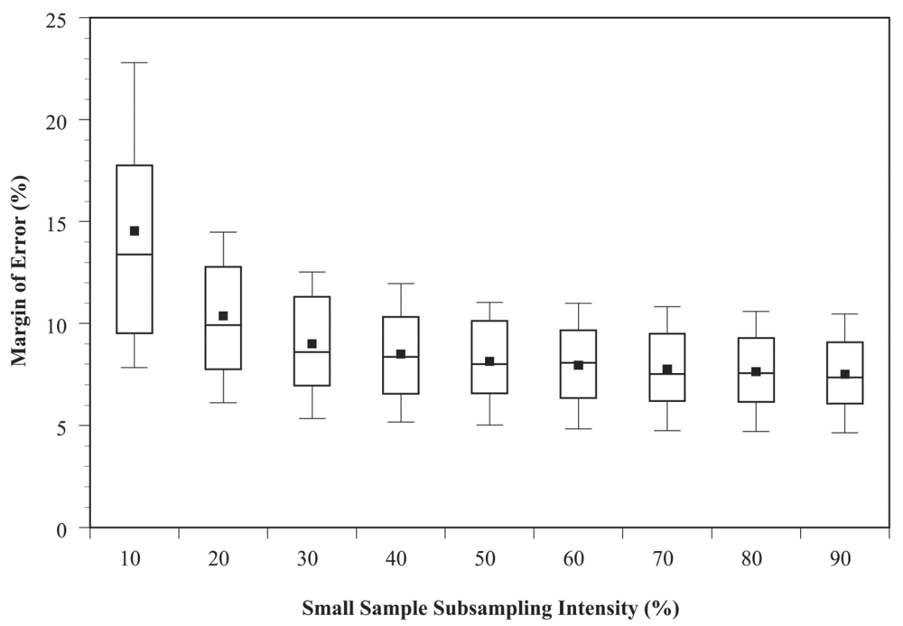
| Relative efficiency (%) | Time saved (%) | |||||||||
|---|---|---|---|---|---|---|---|---|---|---|
| Small sample intensity (%) | Margin of error (%) | Margin of error deviation (%) | 2 to 1 time ratio | 3 to 1 time ratio | 4 to 1 time ratio | 6 to 1 time ratio | 2 to 1 time ratio | 3 to 1 time ratio | 4 to 1 time ratio | 6 to 1 time ratio |
| 100 * | 7.43 | 0 | 100 | 100 | 100 | 100 | 0 | 0 | 0 | 0 |
| 90 | 7.52 | 0.1 | 92 | 93 | 94 | 95 | 5 | 7 | 8 | 8 |
| 80 | 7.64 | 0.22 | 94 | 98 | 100 | 102 | 10 | 13 | 15 | 17 |
| 70 | 7.76 | 0.34 | 97 | 103 | 107 | 110 | 15 | 20 | 23 | 25 |
| 60 | 7.94 | 0.52 | 99 | 108 | 113 | 119 | 20 | 27 | 30 | 33 |
| 50 | 8.15 | 0.72 | 102 | 115 | 122 | 131 | 25 | 33 | 38 | 42 |
| 40 | 8.5 | 1.08 | 102 | 119 | 130 | 143 | 30 | 40 | 45 | 50 |
| 30 | 9.01 | 1.58 | 102 | 124 | 139 | 158 | 35 | 47 | 53 | 58 |
| 20 | 10.37 | 2.95 | 90 | 116 | 135 | 162 | 40 | 53 | 60 | 67 |
| 10 | 14.54 | 7.12 | 68 | 94 | 115 | 150 | 45 | 60 | 68 | 75 |
4. Conclusions
Acknowledgments
Conflict of Interest
References and Notes
- Merten, P.R.; Wiant, H.V.; Rennie, J.C. Double sampling saves time when cruising Appalachian hardwoods. North. J. Appl. For. 1996, 13, 116–118. [Google Scholar]
- Avery, T.E.; Burkhart, H.E. Forest Measurements, 5th ed; McGraw-Hill: New York, NY, USA, 2002; pp. 250–252. [Google Scholar]
- Oderwald, R.G.; Jones, E. Sample sizes for point, double sampling. Can. J. For. Res. 1992, 22, 980–983. [Google Scholar]
- Oderwald, R.G. Stock and stand tables for point, double sampling with a ratio of means estimator. Can. J. For. Res. 1994, 24, 2350–2352. [Google Scholar]
- Oderwald, R.G. Augmenting inventories with basal area points to acheive desired precision. Can. J. For. Res. 2003, 33, 1208–1210. [Google Scholar]
- Jenkins, J.C.; Chojnacky, D.C.; Heath, L.S.; Birdsey, R.A. National-scale biomass estimators for United States tree species. For. Sci. 2003, 49, 12–35. [Google Scholar]
- Woudenberg, S.W.; Conkling, B.L.; O’Connell, B.M.; LaPoint, E.B.; Turner, J.A.; Waddell, K.L. The Forest Inventory and Analysis Database: Database Description and Users Manual Version 4.0 for Phase 2; U.S. Department of Agriculture, Forest Service, Mountain Research Station: Fort Collins, CO, USA, 2009. [Google Scholar]
- Bell, J.F.; Dilworth, J.R. Log Scaling and Timber Cruising; Oregon State University Book Stores, Inc.: Corvallis, OR, USA, 2007; pp. 182–252. [Google Scholar]
- Coble, D.W.; Grogan, J. Comparison of systematic line-point and double sampling designs for pine and hardwood forests in the western gulf. South. J. Appl. For. 2007, 31, 199–206. [Google Scholar]
Appendix 1
| Stand | Area (ha) | Site index (m) | Dbh (cm) | Basal area (m2 ha−1) | Aboveground biomass (mt ha−1) |
|---|---|---|---|---|---|
| 1 | 31.2 | 26 | 29.5 | 17.6 | 117.6 |
| 2 | 32.4 | 24 | 32.3 | 18.8 | 136.1 |
| 3 | 32.8 | 21 | 28.9 | 21.6 | 116.3 |
| 4 | 36.0 | 27 | 31.9 | 22.6 | 160.7 |
| 5 | 49.8 | 25 | 35.8 | 24.9 | 169.1 |
| 6 | 54.2 | 18 | 30.3 | 17.4 | 114.8 |
| 7 | 59.1 | 25 | 29.8 | 21.4 | 144.1 |
| 8 | 78.1 | 24 | 32.0 | 21.9 | 150.6 |
| 9 | 88.2 | 20 | 29.2 | 25.5 | 151.1 |
| 10 | 88.2 | 29 | 28.9 | 21.3 | 139.0 |
| 11 | 99.1 | 22 | 32.1 | 22.7 | 161.1 |
| 12 | 100.0 | 25 | 28.4 | 20.0 | 127.3 |
| 13 | 117.4 | 21 | 32.3 | 19.1 | 136.3 |
| 14 | 119.0 | 20 | 30.1 | 19.3 | 118.8 |
| 15 | 120.2 | 20 | 32.9 | 19.3 | 143.1 |
| 16 | 122.2 | 22 | 30.0 | 19.0 | 131.1 |
| 17 | 146.1 | 21 | 31.8 | 22.5 | 158.8 |
| 18 | 161.5 | 26 | 29.7 | 22.6 | 160.1 |
| 19 | 170.0 | 24 | 28.5 | 24.1 | 151.0 |
| 20 | 173.6 | 22 | 29.4 | 20.2 | 135.8 |
| 21 | 174.8 | 30 | 30.6 | 25.1 | 167.2 |
| 22 | 174.8 | 23 | 34.6 | 22.2 | 159.0 |
| 23 | 177.3 | 25 | 33.2 | 18.4 | 125.6 |
| 24 | 177.3 | 23 | 33.0 | 19.5 | 141.8 |
| 25 | 211.2 | 26 | 30.5 | 21.6 | 148.9 |
| 26 | 219.3 | 22 | 30.6 | 21.1 | 148.4 |
| 27 | 235.1 | 26 | 31.3 | 19.4 | 138.6 |
| 28 | 271.5 | 19 | 29.2 | 22.3 | 140.6 |
| 29 | 300.3 | 20 | 36.0 | 20.7 | 149.4 |
| 30 | 300.7 | 25 | 30.1 | 30.6 | 203.0 |
| 31 | 337.5 | 25 | 35.0 | 22.3 | 150.5 |
| 32 | 348.0 | 23 | 31.9 | 21.3 | 149.0 |
| 33 | 399.4 | 24 | 33.2 | 18.4 | 125.6 |
| 34 | 412.8 | 21 | 28.8 | 21.0 | 143.8 |
| 35 | 478.7 | 24 | 34.1 | 23.2 | 165.7 |
| 36 | 538.2 | 22 | 30.5 | 19.4 | 137.8 |
| 37 | 601.8 | 23 | 30.0 | 20.5 | 142.0 |
| 38 | 625.2 | 23 | 25.7 | 22.1 | 149.2 |
| 39 | 664.5 | 21 | 26.3 | 19.5 | 130.5 |
| 40 | 1155.4 | 23 | 32.3 | 23.3 | 156.3 |
© 2012 by the authors; licensee MDPI, Basel, Switzerland. This article is an open-access article distributed under the terms and conditions of the Creative Commons Attribution license (http://creativecommons.org/licenses/by/3.0/).
Share and Cite
Parrott, D.L.; Lhotka, J.M.; Fei, S.; Shouse, B.S. Improving Woody Biomass Estimation Efficiency Using Double Sampling. Forests 2012, 3, 179-189. https://doi.org/10.3390/f3020179
Parrott DL, Lhotka JM, Fei S, Shouse BS. Improving Woody Biomass Estimation Efficiency Using Double Sampling. Forests. 2012; 3(2):179-189. https://doi.org/10.3390/f3020179
Chicago/Turabian StyleParrott, David L., John M. Lhotka, Songlin Fei, and B. Scott Shouse. 2012. "Improving Woody Biomass Estimation Efficiency Using Double Sampling" Forests 3, no. 2: 179-189. https://doi.org/10.3390/f3020179