1. Introducción
High-resolution (HR) remote sensing images provide detailed texture information of ground objects, which are essential for many applications, such as the classification of land cover [
1], object detection [
2], building extraction [
3], and change detection [
4]. However, the spatial resolution of remote sensing images is influenced by the sensor hardware and environmental factors [
5], and it is relatively difficult to obtain HR images at a specific time. At the hardware level, it is possible to increase the number of satellites to provide more HR satellites or directly improve the production technology of sensors to directly improve the resolution. These options tend to be more costly in most instances. In comparison with the above strategies, super-resolution (SR) image technology is more convenient and of relatively low cost. SR is a technique for generating HR images from low-resolution (LR) images. The approach can be categorized into the single-image super-resolution (SISR) or multi-image super-resolution (MISR). Although the multi-image technique can provide more a priori information, it is difficult to obtain multiple remote sensing images of the same scene.
The traditional image SR algorithms can be grouped into two main categories, interpolation-based algorithms, and reconstruction-based algorithms. The interpolation-based image SR methods reconstruct HR images by computing the pixels of the point to be sought from the known pixel values around the point to be interpolated. The main commonly used interpolation algorithms include the nearest neighbor interpolation [
6], the bilinear interpolation [
7], and the bicubic interpolation [
8] methods. Interpolation algorithms tend to be faster and simpler than other methods. However, linear model algorithms have limited ability to recover high-frequency detail. Reconstruction-based algorithms use complex a priori knowledge as constraints to reconstruct the HR images, such as iterative back projection (IBP) [
9], projection onto convex sets (POCS) [
10], and maximum-a-posteriori (MAP) approach [
11]. Although reconstruction-based algorithms utilize a priori information, they do not always generate acceptable results for complex images.
In recent years, with the development of deep learning techniques, a series of deep learning-based methods have emerged in the field of SR. Dong et al. [
12] proposed a super-resolution convolutional neural network (SRCNN), which learns the mapping relationship between bicubic linear interpolation images and HR images through the use of neural networks. Although the SRCNN can outperform traditional-based methods, bicubic LR images are computationally slow in the network. To alleviate the problem, a fast super-resolution convolutional neural network (FSRCNN) [
13] has added transposed convolution operations to the network to reduce the computational time of the network. These networks are shallow, and their performance is affected by the depth of the network; however, increasing the depth of the network can lead to gradient explosion and gradient disappearance. To deepen the depth of the network and obtain a stronger learning ability, very deep super-resolution (VDSR) [
14] incorporates residual learning and gradient cropping to mitigate the network gradient explosion-disappearance problem. Further, the use of the deeply recursive convolutional network (DRCN) [
15] increases the network depth skip connections and recursive supervision. Additionally, the deep recursive residual network (DRRN) [
16] improves the performance of the network by proposing recursive learning of local residual connections and residual units on the basis of the DRCN. Moreover, enhanced deep super-resolution (EDSR) [
17] and SRResNet [
18], which use residual connections [
19], deepen the network depth and avoid the gradient problem. EDSR removes the batch normalization (BN) [
20] layer and uses a residual scaling module to increase the stability of the training.
In previously reported networks, all the different channels are characterized and treated equally, and the residual channel attention network (RCAN) [
21] uses channel attention to enhance the ability of the network to distinguish between the different channels. The dual regression network (DRN) [
22] proposes a dual regression scheme by introducing an additional constraint on the LR data to reduce the space of the possible functions. The local texture estimator (LTE) [
23] proposes an LTE, a dominant-frequency estimator for natural images, enabling an implicit function to capture fine detail while reconstructing images in a continuous manner. To reduce the amount of computation in the SR network, sparse mask SR (SMSR) [
24] is adopted to learn sparse masks to prune redundant computation. In addition to the CNN-based models, the transformer [
25] model has been used in the field of SR due to its excellent global attention mechanism and texture transformer network (TTSR) [
26]. The TTSR uses the LR and the reference image (Ref) as a query and a keyword. Joint feature learning is then performed between the LR and the Ref to extract the relationship between the deep features by global attention, and thus the texture features are displayed accurately. Although the transformer can obtain the global receptive field, the computational effort increases rapidly with image size [
27]. Liang et al. [
28] used a Swin transformer [
29] for deep feature extraction to reduce the computational effort in computing attention. To activate more input pixels for reconstruction, the hybrid attention transformer (HAT) [
30] was adopted, combining channel attention and self-attention schemes, which exploit the respective complementary advantages.
CNN and transformer-based methods achieve better recovery results compared to the traditional SR methods, but the recovered images are sometimes too smooth and lack high-frequency detail. Compared to these methods, the generating adversarial network (GAN) based SR method is able to produce more detailed textures. The GAN consists of a generator and a discriminator. The generator generates an image from the input, the discriminator determines whether the generated image is true or false, and then alternately is optimized to reach the Nash equilibrium [
31]. The super-resolution generative adversarial network (SRGAN) [
18] uses GAN to solve the SR problem and proposes a perceptual loss to produce more realistic textures. The enhanced super-resolution generative adversarial network (ESRGAN) [
32] improves the discriminator using the relativistic average GAN (RaGAN) [
33] and introduces the residual-in-residual dense block (RDDB) to improve the model. The spatial feature transforms generative adversarial network (SFTGAN) [
34] uses an SFT module to effectively combine the images into the network to improve detailed texture in the GAN networks. The Real-ESRGAN [
35], a high-order degradation modeling process, is introduced to better simulate complex real-world degradations and employs a U-Net discriminator with spectral normalization to increase the discriminator capability and stabilize the training dynamics.
In addition to improvements in the model itself, research on the degradation of the HR-LR has been a hot topic in recent years. The super-resolution network for multiple degradations (SRMD) [
36] proposes a general framework featuring a dimensionality stretching strategy that enables a single convolutional SR network to take two key factors of the SISR degradation process, that is, the blur kernel and the noise level, as the inputs. A unified dynamic convolutional network (UDVD) [
37] introduces a dynamic convolution based on the SRMD and applies dynamic convolution to the up-sampling process. Iterative kernel correction (IKC) [
38] solves the artifacts caused by kernel mismatch by correcting the estimated blur kernels through an iterative correction mechanism. Inspired by contrast learning, domain adaptation super resolution (DASR) [
39] is proposed as an unsupervised degradation-aware network, which is based on representation learning, to handle different degradation situations adaptively. The unpaired SR [
40] proposes a probabilistic degeneracy model (PDM) that studies the degeneracy D as a random variable and learns its distribution by modeling the mapping from a priori random variables Z to D. Blind image super-resolution with elaborate degradation modeling (BSRDM) [
41] proposes a patch-based noise model to increase the degrees of freedom of the model for noise representation and to facilitate novel construction of a concise yet effective kernel generator.
The SR has become a research hotspot in image processing in remote sensing due to the huge demand for high spatial resolution in many remote sensing tasks. Jiang et al. [
42] proposed the distillation recursive network (DDRN) for video satellite image SR. Galar et al. [
43] used the EDSR with several modifications on Sentinel-2 and Planet images. Romero et al. [
44] implemented and trained a model based on ESRGAN with pairs of WorldView-Sentinel images to generate a super-resolution multi-spectral Sentinel-2 output with a scaling factor of 5. Zabalza et al. [
45] exploited the residual network (SARNet) to increase the spectral resolution of the Sentinel-2 images from the original 10 m to 2.5 m. Karwowska et al. [
46] improved the resolution of satellite images acquired with the World View 2 satellite using the ESRGAN network with window functions.
Although the above-mentioned methods deliver good performance, there is still scope for improvement in the remote sensing image SR mission. First, the real degradation of remote sensing images is very complex, given that the process involves the diffraction limit of the lens, disturbances by the atmosphere, the relative movement of the imaging platforms, and the impacts of the different types of imaging noise. All these factors lead to difficulties in producing valid results for real remote sensing images, even for models that consider multiple degradations [
47,
48]. Therefore, ground truth data are very important for SR in remote sensing images. However, there are few studies on real ground truth data with high spatial resolution, especially at the meter scale. Second, the GAN network can produce more high-frequency information. Nonetheless, adversarial training is unstable and often produces unpleasant visual artifacts, which is a problem exacerbated by the complexity of the remote sensing image distribution. Third, the remote sensing images are complex and contain detailed and rich information. This both generates difficulties in the SR of remote sensing images and provides more a priori information. The existing GAN networks do not focus on the similarities and differences in this information.
To solve these problems, an SR dataset of real remote sensing images was built using different spatial resolutions for the Gao Fen (GF) satellite data, whereby a GAN model based on second-order channel attention and a region-level non-local module is proposed to utilize the rich a priori information of remote sensing images, and finally, use a region-aware strategy to inhibit the generation of artifacts.
The main contributions of this study are as follows:
A real SR dataset based on GF6/1 and GF2/7 satellite data is produced to simulate the degradation process of real remote sensing images.
A region-aware strategy is added to the training process to reduce the artifacts generated in GAN and improve the visual quality of the results.
An adversarial generative network for SR reconstruction of real remote sensing images was designed, whereby a second-order channel attention mechanism was used to treat channel features differently. A region-level non-local module was added to the generative network to capture long-range dependencies between features, which achieved an accurate restoration of feature structure information.
The paper is organized as follows: The proposed SR method is introduced in detail in
Section 2. The evaluation experiments for the different methods are described in
Section 3. A further discussion of the proposed method is given in
Section 4. Finally, future research directions are specified in the conclusions in
Section 5.
3. Results
In this section, the commentary is given on the following topics: the proposed dataset, comparison with other current state-of-the-art models, ablation experiments, spectral validation, and migration experiments.
3.1. Dataset
In previous studies, most datasets were produced by adding noise and blur to the down-sampled HR images to realize paired LR-HR image pairs, but the trained datasets based on this approach are often poor in terms of recovery in the real remote sensing images. To solve this problem, this study did not use publicly available datasets but built SR datasets based on four bands (red band, green band, blue band, and NIR band) GF satellite data with different spatial resolutions so that the model can learn more complex mapping relationships. The dataset consists of data from satellites GF7, GF2, GF1, and GF6, and the spatial resolution of each satellite is shown in
Table 1.
Satellite data were selected from four regions in China, that is, Beijing, Ordos, Guangzhou, and Fuzhou. In terms of time, to minimize the influences of environmental change, LR and HR images with similar times as possible were selected, of which the satellites used in each region and the times are shown in
Table 2.
We first performed a radiometric correction based on the calibration coefficients of the GF satellites. An improved OptVM [
62] is applied for band fusion. It can produce a high-resolution panchromatic image from a low-resolution multi-spectral image automatically. Afterward, the SIFT feature constraint optical flow method (SIFT-OFM) [
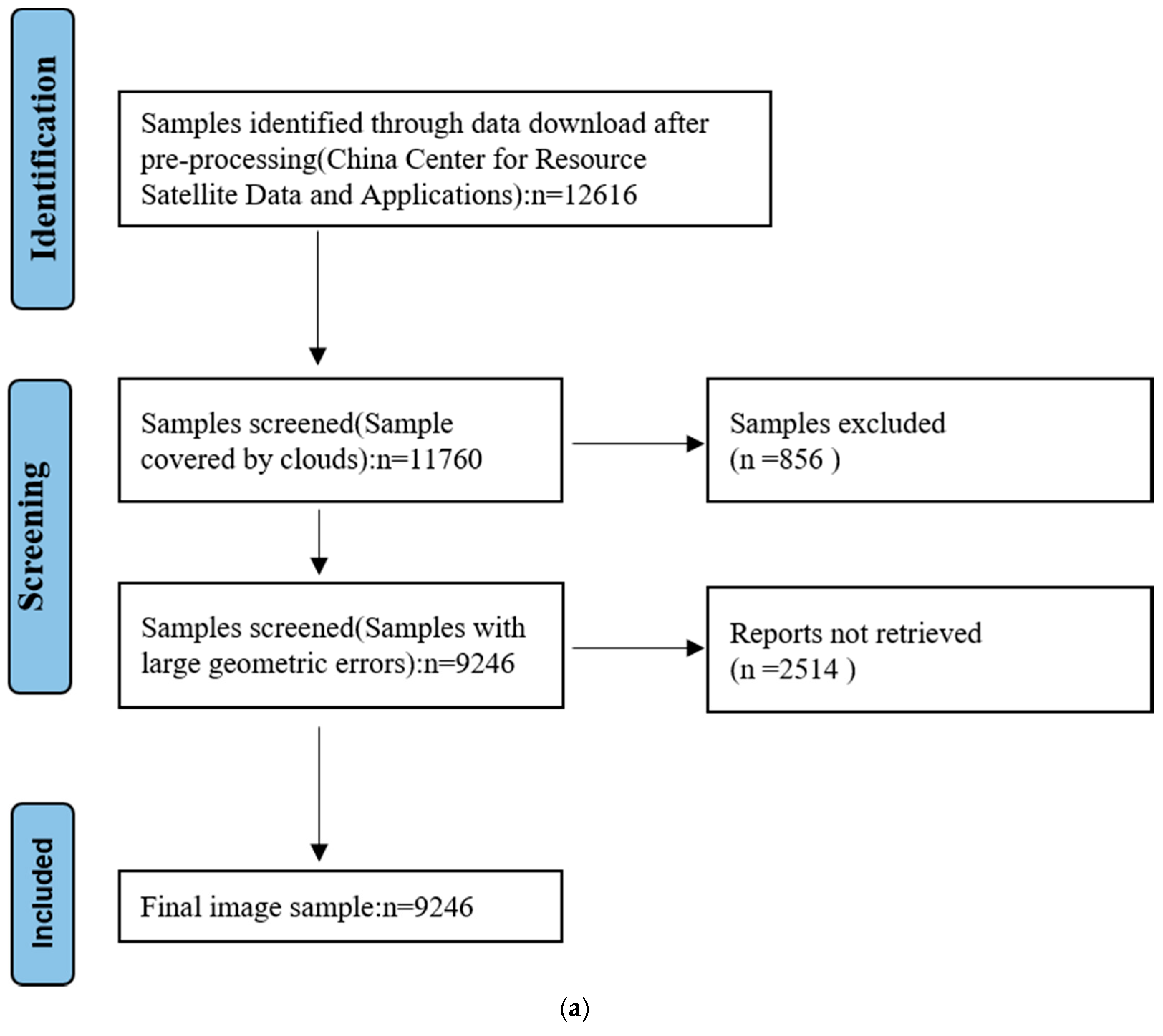
62] is used to register images. Given that the spatial resolution of the HR image was 0.8 m, the existing model can only super-resolve the image by an integer multiple, while the spatial resolution of the LR image is 2 m; therefore, we down-sampled the HR image to 1 m by using a cubic function. Opencv2 was then used to crop the HR and LR images to 200 × 200 and 100 × 100, respectively, according to the latitude and longitude. A total of 9246 image pairs were finally generated. The images were divided randomly, with 90% serving as the training data and 10% as the validation data. The PRISMA diagram for sample identification in the study is shown in
Figure 8a, and the final resulting dataset is shown in
Figure 8b.
3.2. Training Details
The network is composed of two parts, the discriminator network and the generator network. The discriminator network consists of five basic blocks, and each block includes a convolutional layer responsible for feature extraction, a convolutional layer for feature map size reduction, and a BN layer where the input feature map size is 100 × 100. The generator part consists of 23 RRDCB blocks, and the number of input channels in each RRDCB block is 64; the growth of each channel in the RRDCB internal layer is 32. The generator and discriminator optimizers are based on the work of Adam [
50].
During the training process, the input LR-HR image pairs are cropped randomly into 50 × 50 and 100 × 100 and subjected to data enhancement operations such as horizontal flip, vertical flip, and rotation. The PyTorch framework is employed to train on two Nvidia A4000 chips with a memory size of 16 GB. Further details of the experiments are given in
Table 3.
3.3. Evaluation Metrics
The peak signal-to-noise ratio (PSNR) [
63], the structural similarity (SSIM) [
64], the Frechet inception distance score (FID) [
65], and the learned perceptual image patch similarity (LPIPS) [
66] were selected as the evaluation metrics. The PSNR gives a measure of the degree of distortion by calculating the squared pixel-by-pixel difference between the LR and HR images; a larger PSNR value indicates that the two images are more similar. The PSNR is calculated as follows:
where
is the maximum value of pixels in the image, and the
is given by:
SSIM gives a measure of the similarity of an image by comparing the brightness, contrast, and structure of the two images; the larger the SSIM value, the better the result for image recovery. The formula for calculating the SSIM is given by Equation (34).
The PSNR and SSIM are traditional metrics for the evaluation of image quality; however, there are two problems with using only PSNR and SSIM for evaluation. First, the PSNR and SSIM do not truly reflect the quality of the images of some scenes, and higher values do not necessarily represent better quality, as is demonstrated below in the visualization of the structure. Second, the model adopted in this study is based on generative adversarial networks, and the PSNR and SSIM do not consider the relationship between the direct probability distribution of the generated samples and the real samples. Hence, the FID and LPIPS have been included in the suite of metrics to evaluate the quality of image recovery.
The FID is a metric to calculate the distance between the real image and the feature vectors of the generated image. It was shown to correlate well with the human judgment of visual quality and is most often used to evaluate the quality of samples of generative adversarial networks. FID is calculated by computing the Fréchet distance between two Gaussians fitted to feature representations of the Inception network. The higher the quality of image generation, the FID is calculated as follows:
where
represents the square of
parametrization;
(.
represents the trace of the matrix;
are the means of the real image feature vector and the generated image, respectively;
are the variances of the real image feature and the generated image feature, respectively.
The LPIPS uses a VGG network to extract features from the generated image and the real image and evaluates the similarity between the two images by measuring the square of the
the parametric number between the generated image features as well as the real image features, systematically evaluate deep features across different architectures and tasks. The value for the LPIPS is calculated as follows:
where
represent the features of the lth feature layer of the generated image and the real image, and
is a preset value for the lth feature layer weight. The smaller the LPIPS value, the more similar the generated image is to the real image.
3.4. Comparison with Existing Models
In this study, the bicubic, the super-resolution residual network (SRResNet), the enhanced deep super resolution (EDSR), the residual channel attention network (RCAN), the super-resolution generative adversarial network (SRGAN), and the enhanced super resolution generative adversarial network (ESRGAN) are used in comparison analyses with the proposed model, in which 16 residual blocks are used in the SRResNet, and the number of channels of feature maps within each residual block is 64; the EDSR uses 32 residual blocks, and the number of channels in each residual block is 256; the RCAN uses 10 RCAB groups consisting of RB basic blocks, and each RCAB group includes 20 RB blocks and the number of channels in each basic block is 64; the SRGAN has the same generator configuration as the SRResNet, the discriminator uses the VGG network where the depth of the VGG is 5, and the number of input channels to the discriminator is 64; the generator of the ESRGAN consists of 23 RRDB blocks, the number of feature channels within each basic block is 64, the number for channel growth is set to 32, each block includes five dense residual connected convolutional layers, and the discriminator is the same as for the SRGAN. These methods are retrained on our proposed dataset to achieve a fair comparison network, and the number of input channels for the discriminator is 64; moreover, to allow a fair comparison, these methods are retrained on the training set of our proposed dataset and tested on the test set.
The values of the PSNR, SSIM, LPIPS, and the FID of the model in the validation dataset after 450,000 iterations are presented in
Table 4.
As can be seen in
Table 4, the EDSR achieves the best value for the PSNR and the SSIM metrics, while all the CNN models significantly outperform the GAN in terms of metrics, mainly because both the PSNR and the SSIM are computed using simple relationships between the pixel values of the image, which is similar to the definition of the loss function in the CNN networks; however, the proposed method achieves greater improvements in both metrics compared to the GAN-based methods. With respect to the PSNR and the SSIM, our model is only lower than the EDSR model by 0.7325 DB and 0.0344 DB, respectively. Our model achieves the best results for LPIPS and FID, and contrary to the previous, the GAN-based model outperforms the CNN-based model on these two metrics; moreover, the proposed method is 0.05 and 1.1695 lower than the second-ranked method on the LPIPS and FID, respectively.
In
Figure 9, it can be seen that the CNN-based approach tends to generate results that are too smooth, while the GAN-based approach is able to generate more detail. Compared with other GAN-based methods, the visual quality of the present method is also the best. From the visualization results, our model has three advantages. First, we are able to produce more detail. As shown in
Figure 9a, the proposed method has a clearer and sharper reduction in zebra lines, and in
Figure 9b, there is a more accurate reduction in the container edges. Second, the second-order attention mechanism makes the color reproduction of the feature more accurate; as in
Figure 9b, the color reproduction is closer to the original image. Third, with the help of the region-aware strategy, our image produces fewer artifacts; as can be seen in
Figure 9c, the other two GAN-based methods display incorrect textures on some houses, whereas in the present method, it can basically restore the real situation of the houses correctly. Moreover, in
Figure 9d, the other methods present a coarser restoration of the blue roof (see below), while our method is smoother and conforms to the HR image. In addition, from the visualization results, it can be concluded that the FID and LPIPS metrics are more in keeping with the public’s perceptions compared to the PSNR and the SSIM.
3.5. Ablation Study
To illustrate the effectiveness of the modifications, the results of several ablation experiments are considered. We gradually add region-aware strategies, second-order attention mechanisms, and region-level non-local modules to the baseline model and train them with the same configuration and test them on the validation set. The comparison data for each metric are presented in
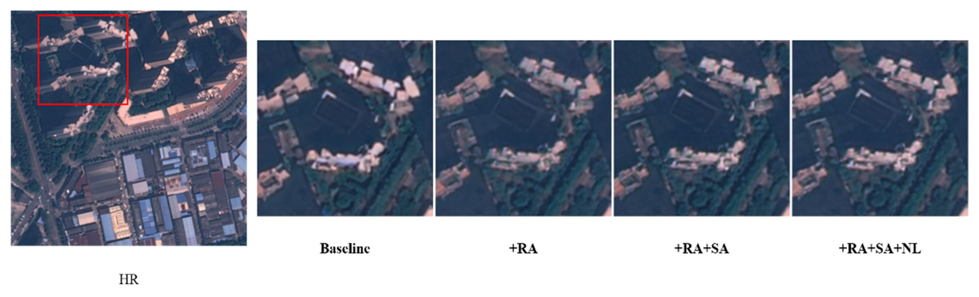
Table 5, and the entire visualization process is shown in
Figure 10.
As can be seen from
Table 5, the metrics of the model improve overall when adding different modules, and where the model used in this study delivers the best performance of all the metrics with the exception of the LPIPS. The three improvements are ordered in descending order of influence as region-aware strategy, second-order channel attention mechanism, and region-level non-local module, compared to the baseline model. The model used in this work delivers the best performance in terms of the PSNR, the SSIM, the FID, and the LPIPS, the metrics being improved by 7.64%, 16.61%, 17.67%, and 6.11%, respectively. However, the LPIPS value did not improve after adding the region-level non-local module. It is considered that the NL is less appropriate for applying to the LPIPS. The LPIPS values are calculated by extracting high-level features from the network, while the non-local module is more helpful for the reconstruction of spatial information, such as edges, textures, etc., which are low-level features. In addition, high-level features are generally more concerned with global information, while low-level features are more concerned with local information; thus, there is no direct correlation between them. Our non-local module only computes in local regions of the images to reduce the computation time. The combination of the above factors causes a small decrease in the LPIPS.
As shown in
Figure 10, the baseline model has a light blue artifact for the roof. After adding the region-aware strategy, the artifact disappears, and more detailed information is generated at the same time. However, the color of the building roof becomes grayish, while in the HR image, it is white. After adding the second-order channel attention mechanism, the roof color reverts to white, as observed in the HR image. Finally, by adding the non-local module, the outer contour of the building is more accurate, and at the same time, the roof becomes smoother.
3.6. Spectral Validation
In addition to visual enhancement, when further applying SR images, we need to ensure that the reflectance values are similar to those of real LR or SR satellite images. In this section, analysis was undertaken to verify that the spectral content of the SR image was similar to the real image under the different preprocessing scenarios.
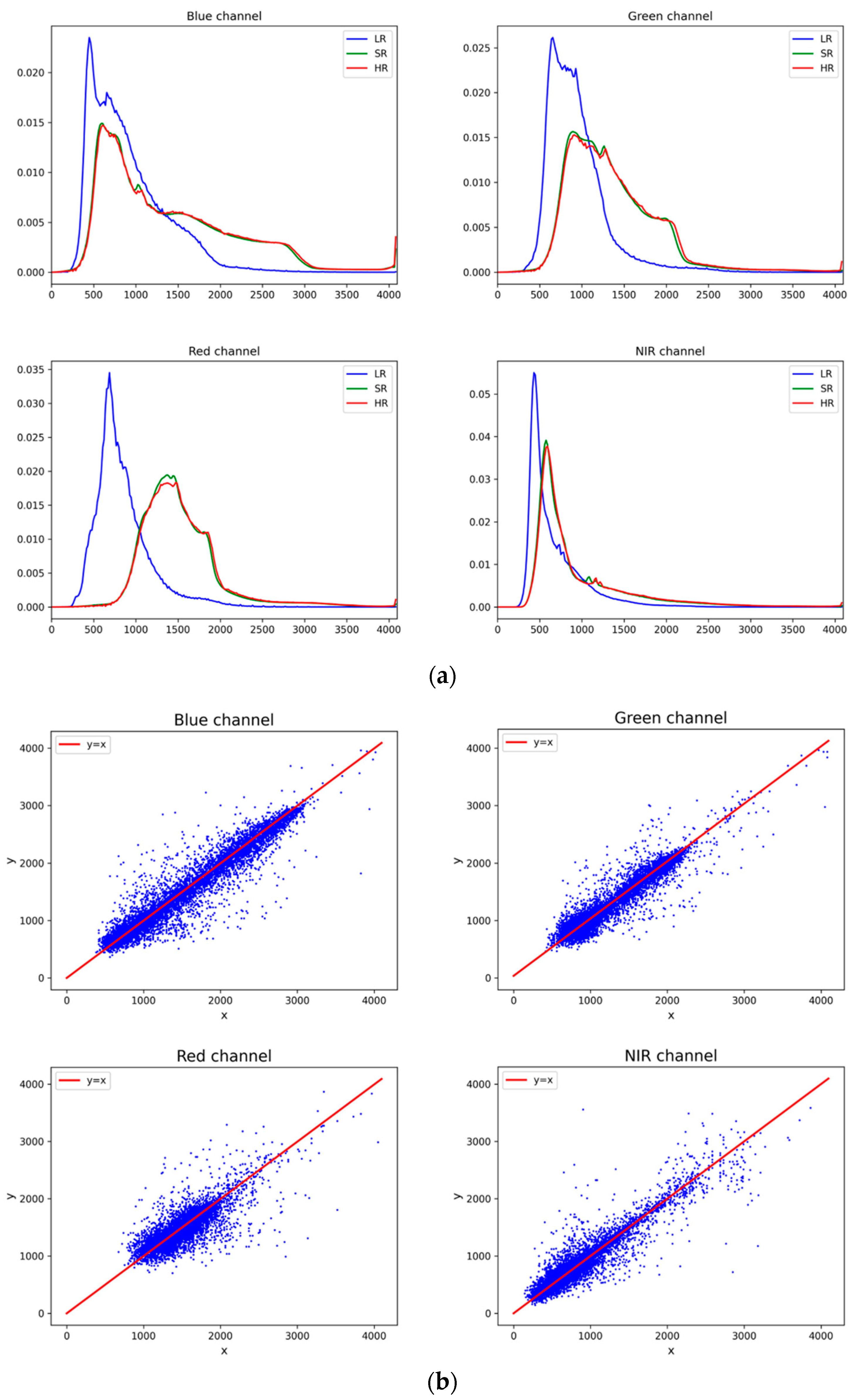
The LR, HR, and SR histograms of an image from a test set are presented in
Figure 11a. As can be seen, the histogram of the SR image is more similar to the HR image, which indicates that the proposed model learns the spectral information of the HR image through training. The reflectance values of 10,000 randomly selected pixels from the test data from HR and SR images are plotted in
Figure 11b. From the scatter plot, an extremely strong correlation between SR images and HR images can also be found.
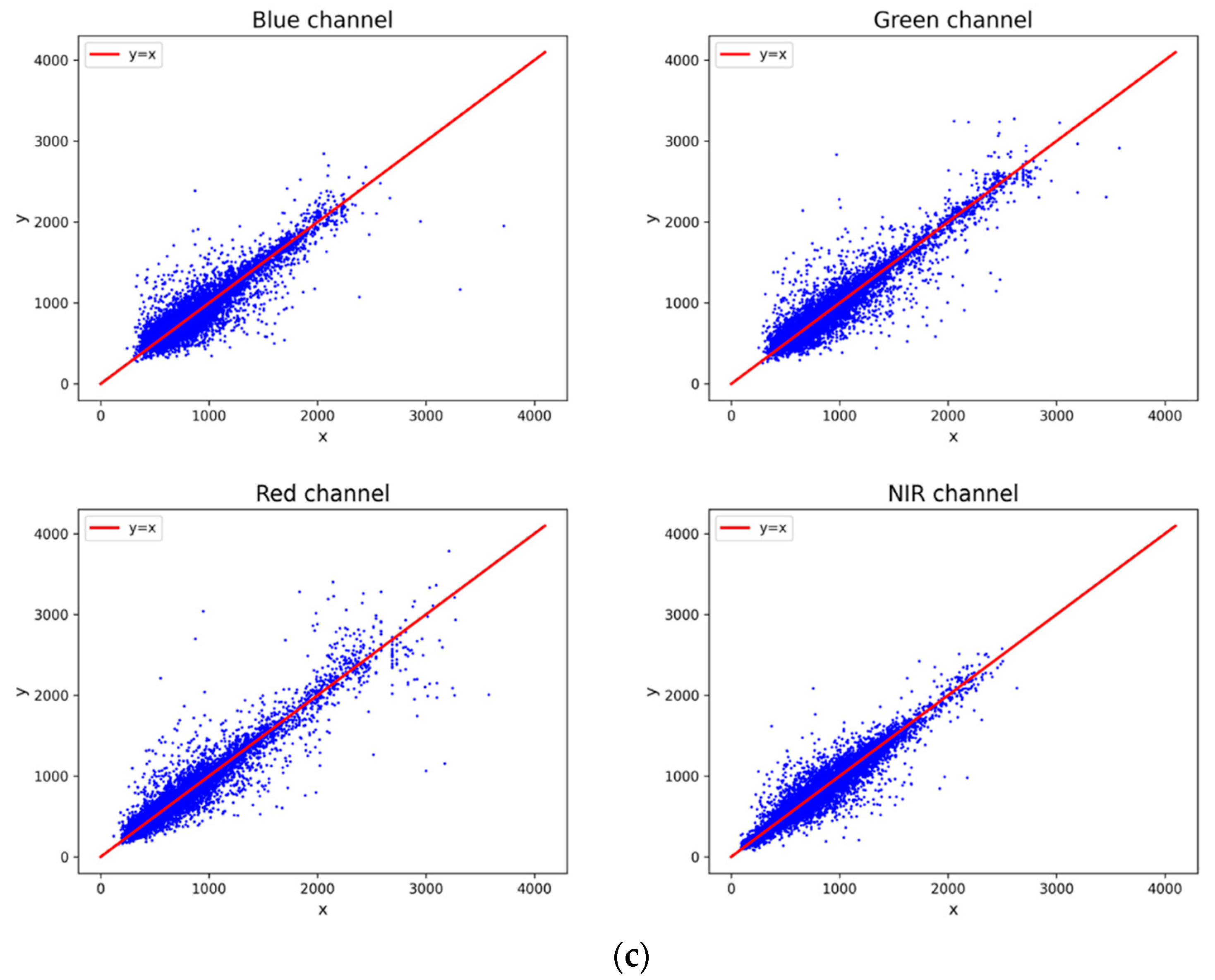
However, the spectral characteristics of both SR images and HR images are significantly different from those of LR images. We believe this is due to sensor differences between satellites. Further, to verify that the model also has the ability to retain the spectral information of the LR images. We reprocessed the images of the Guangzhou area; in addition to the preprocessing in
Section 3.1, the relative radiometric correction using the histogram matching was performed on the HR images and LR images with Sentinel-2 images as the reference in the same period, and experiments were conducted on the respective test sets. As shown in
Figure 12, after relative radiation corrected LR, HR and SR images have similar colors. SR images also obtained by the model can also retain the spectral information of the LR images well as a result of the additional preprocessing. Further, the reflectance values showed a strong correlation. The above experimental model can maintain the LR spectral information.
3.7. Migration Experiments
In this section, the proposed model is used to enhance the spatial resolution of the GF1 satellites from 2 m to 1 m. The datasets originate from the GF1B satellite image of Beijing on 21 October 2021 and the GF1D satellite image of Hanzhong, Shaanxi Province, on 6 July 2022. The migration experiments for the two-view remote sensing images verify the robustness of the model in time as well as in area.
The left column in
Figure 13 represents the original whole-view image as well as the whole-view image after SR, where the red-rectangle regions and the zoom-in can be further visualized in terms of the local details within each area. The SR results reveal that the proposed method performs well in terms of visual quality. From the visualization results it can be seen that the edges of the image after SR are enhanced, and the information detail is enriched, thus confirming the excellent visual performance of the model in processing real-world data.
4. Discussion
In this study, we constructed an SR dataset of GF satellite images at various spatial resolutions to simulate a real degradation process. Previously reported models were improved, and related experiments were performed. The results in
Section 3.4 and
Section 3.5 demonstrated that the proposed model exhibited good performance on the validation dataset. Moreover, the model outperformed all GAN-based models with respect to both the evaluation metrics and the visual aspects. In addition, we discussed the experimental results in combination with theoretical analysis.
(1) Impact of region-aware strategy: The region-aware strategy locates artifacts by taking the variance of the residual map as the basis while using the EMA. Theoretically, the variance of the artifacts on the SR and the residuals of the HR images should be larger. The smaller variance values indicated that the SR images have an identical deviation in pixel values compared to the HR images, and this only causes the wrong color to be displayed. Therefore, the small variance values in certain regions should not be judged as artifacts. The experimental results are also consistent with the aforementioned conjecture. As shown in
Table 4, the new strategy can significantly improve the performance of the model, and the visualization results from
Figure 9 illustrate that the artifacts can be reduced in both detail-rich regions and smooth regions, thus confirming the effectiveness of the strategy.
(2) Impact of the second-order channel attention mechanism: The second-order channel attention provides more a priori information through normalization of the covariance matrix of the feature map, allowing the network to adjust the channel weights adaptively. Its main impact is a more accurate representation of the color. As can be seen in
Table 4, the method can effectively improve the performance indicators. The visualization results of
Figure 9 and
Figure 10 show that this mechanism has an important role in the accurate restoration of the color of the image.
(3) Impact of the region-level non-local module: The region-level non-local module can calculate the dependency of the features that make full use of similar features in the neighboring region. It can be seen in
Table 4 that the method improves the metrics other than the LPIPS. From inspection of the visualization results in
Figure 9 and
Figure 10, it can be seen that this module can help in the restoration of feature contours.
(4) Comparison with other models: Compared to CNN-based approaches such as EDSR and RCAN, our model produces richer textures through adversarial learning; compared to SRGAN and ESRGAN, our method reduces the generation of artifacts while restoring color and structural information more accurately. Furthermore, most previous studies based on real satellite data used sentinel satellites [
44,
45,
46], while we demonstrate the feasibility of the SR task at the meter level resolution by using GF satellites.
(5) Limits of method: First, the error in the geometric correction of the training data is basically within five pixels. If the error is too large, it will have an impact on the performance of the model. Second, due to the difference in the solar altitude angle, some higher buildings produce huge deviations in images of different spatial resolutions, and this affects the model accuracy to some extent. Third, the SOCA module calculates the covariance matrix and the eigenvalue decomposition process with high time complexity, which leads to a slow calculation speed when the input image or the number of input bands is too large.


