1. Introduction
Rocks are a fundamental component of Earth. They contain the raw materials for virtually all modern construction and manufacturing and are thus indispensable to almost all the endeavors of an advanced society. In addition to the direct use of rocks, mining, drilling, and excavating provide the material sources for metals, plastics, and fuels. Natural rock types have a variety of origins and uses. The three major groups of rocks (igneous, sedimentary, and metamorphic) are further divided into sub-types according to various characteristics. Rock type identification is a basic part of geological surveying and research, and mineral resources exploration. It is an important technical skill that must be mastered by students of geoscience.
Rocks can be identified in a variety of ways, such as visually (by the naked eye or with a magnifying glass), under a microscope, or by chemical analysis. Working conditions in the field generally limit identification to visual methods, including using a magnifying glass for fine-grained rocks. Visual inspection assesses properties such as color, composition, grain size, and structure. The attributes of rocks reflect their mineral and chemical composition, formation environment, and genesis. The color of rock reflects its chemical composition. For example, dark rocks usually contain dark mafic minerals (e.g., pyroxene and hornblende) and are commonly basic, whereas lighter rocks tend to contain felsic minerals (e.g., quartz and feldspar) and are acidic. The sizes of detrital grains provide further information and can help to distinguish between conglomerate, sandstone, and limestone, for example. The textural features of the rock assist in identifying its structure [
1] and thus aid classification. The colors, grain sizes, and textural properties of rocks vary markedly between different rock types, allowing a basis for distinguishing them [
2]. However, the accurate identification of rock type remains challenging because of the diversity of rock types and the heterogeneity of their properties [
3] as well as further limitations imposed by the experience and skill of geologists [
4]. The identification of rock type by the naked eye is effectively an image recognition task based on knowledge of rock classification. The rapid development of image acquisition and computer image pattern recognition technology has thus allowed the development of automatic systems to identify rocks from images taken in the field. These systems will greatly assist geologists by improving identification accuracy and efficiency and will also help student and newly qualified geologists practice rock-type identification. Identification systems can be incorporated into automatic remote sensing and geological mapping systems carried by unmanned aerial vehicles (UAVs).
The availability of digital cameras, hand-held devices and the development of computerized image analysis provide technical support for various applications [
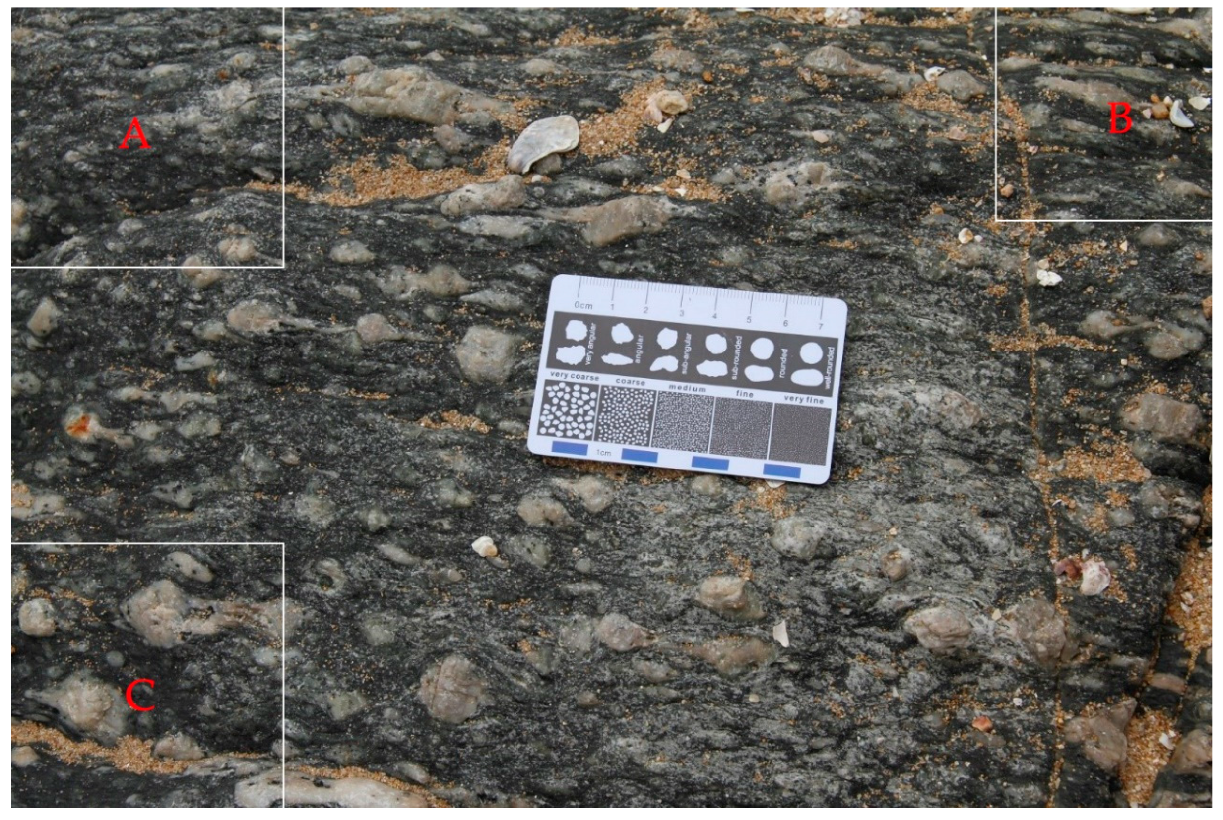
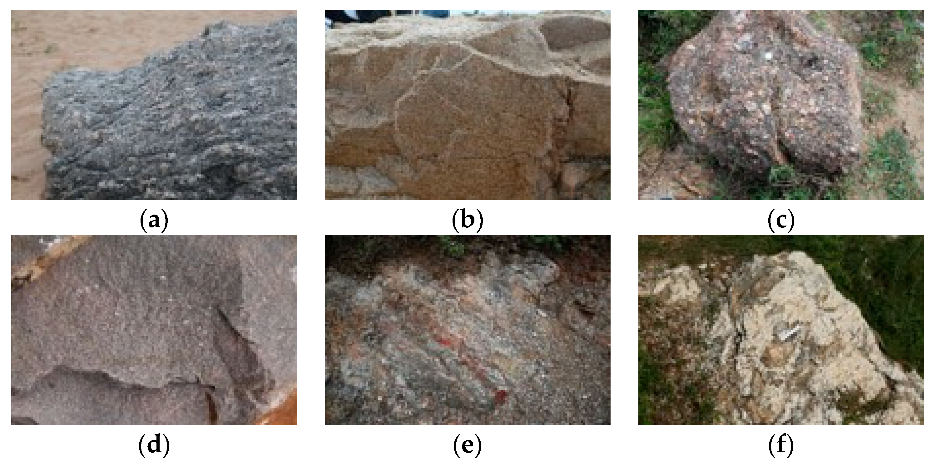
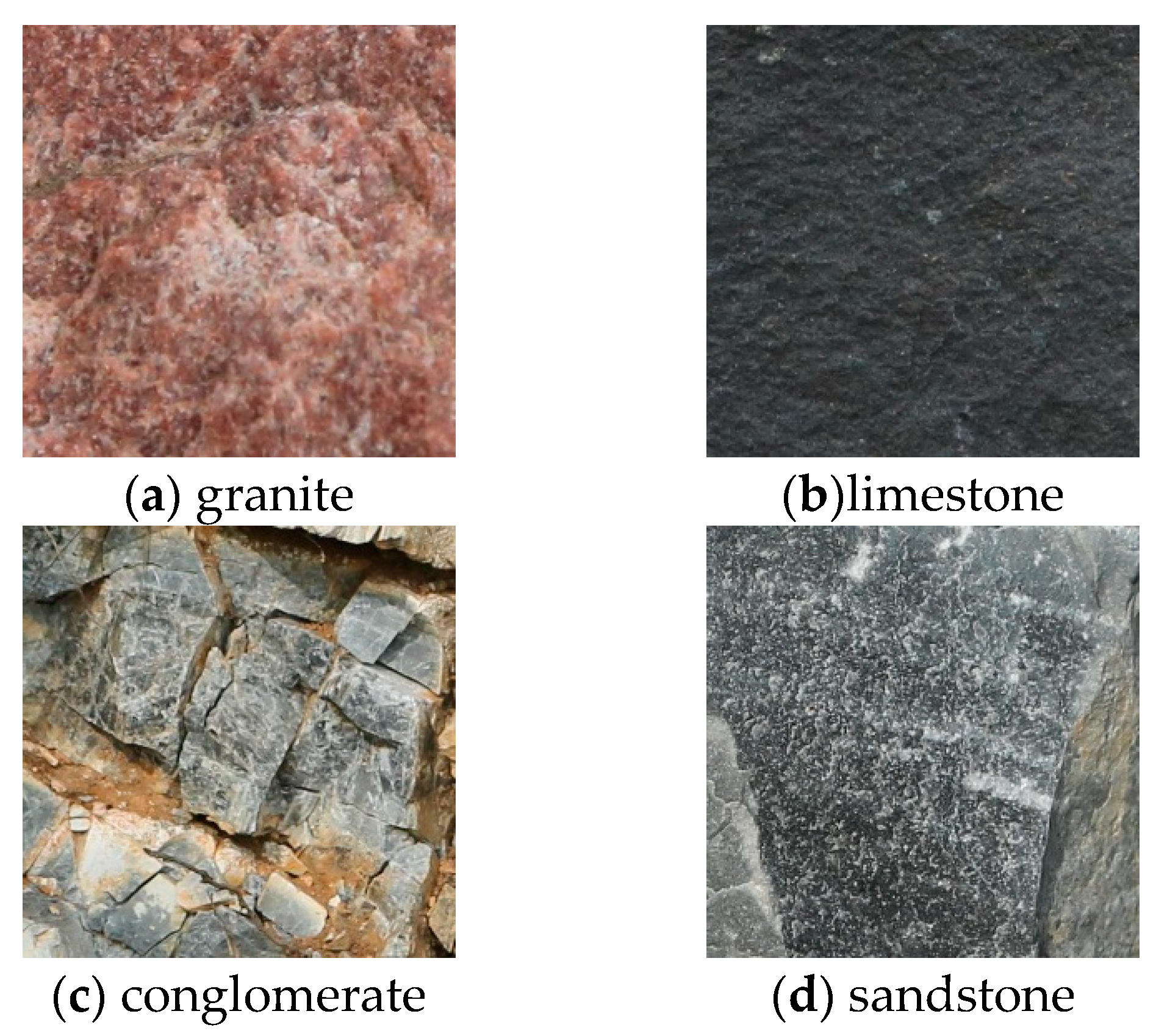
5], so, they allow several characteristics of rocks to be collected and assessed digitally. Photographs can clearly show the characteristics of color, grain size, and texture of rocks (
Figure 1). Although images of rocks do not show homogeneous shapes, textures [
1,
6], or colors, computer image analysis can be used to classify some types of rock images. Partio et al. [
7] used gray-level co-occurrence matrices for texture retrieval from rock images. Lepistö et al. [
6] classified rock images based on textural and spectral features.
Advances in satellite and remote sensing technology have encouraged the development of multi-spectral remote sensing technology to classify ground objects of different types [
8,
9], including rock. However, it is expensive to obtain ultra-high-resolution rock images in the field with the use of remote sensing technology. Therefore, the high cost of data acquisition using hyperspectral technology carried by aircraft and satellites often prevents its use in teaching and the automation of rock type identification.
Machine learning algorithms applied to digital image analysis have been used to improve the accuracy and speed of rock identification, and researchers have studied automated rock-type classification based on traditional machine learning algorithms. Lepistö et al. [
1] used image analysis to investigated bedrock properties, and Chatterjee [
2] tested a genetic algorithm on photographs of samples from a limestone mine to establish a visual rock classification model based on imaging and the Support Vector Machine (SVM) algorithm. Patel and Chatterjee [
4] used a probabilistic neural network to classify lithotypes based on image features extracted from the images of limestone. Perez et al. [
10] photographed rocks on a conveyor belt and then extracted features of the images to classify their types using the SVM algorithm.
The quality of a digital image used in rock-type identification significantly affects the accuracy of the assessment [
2,
4]. Traditional machine learning approaches can be effective in analyzing rock lithology, but they are easily disturbed by the selection of artificial features [
11]. Moreover, the requirements for image quality and illumination are strict, thus limiting the choice of equipment used and requiring a certain level of expertise on the part of the geologist. In the field, the complex characteristics of weathered rocks and the variable conditions of light and weather, amongst others, can compromise the quality of the obtained images, thus complicating the extraction of rock features from digital images. Therefore, existing available methods are difficult to apply to the automated identification of rock types in the field.
In recent years, deep learning, also known as deep neural networks, has received attention in various research fields [
12]. Many methods for deep learning have been proposed [
13]. Deep convolutional neural networks (CNNs) are able to automatically learn the features required for image classification from training-image data, thus improving classification accuracy and efficiency without relying on artificial feature selection. Very recent studies have proposed deep learning algorithms to achieve significant empirical improvements in areas such as image classification [
14], object detection [
15], human behavior recognition [
16,
17], speech recognition [
18,
19], traffic signal recognition [
20,
21], clinical diagnosis [
22,
23], and plant disease identification [
11,
24]. The successes of applying CNNs to image recognition have led geologists to investigate their use in identifying rock types [
8,
9,
25], and deep learning has been used in several studies to identify the rock types from images. Zhang et al. [
26] used transfer learning to identify granite, phyllite, and breccia based on the GoogLeNet Inception v3 deep CNNs model, achieving an overall accuracy of 85%. Cheng et al. [
27] proposed a deep learning model based on CNNs to identify three types of sandstone in image slices with an accuracy of 98.5%. These studies show that CNNs have obtained good results when applied to geological surveying and rock-type recognition. Deep CNNs can identify rock types from images without requiring the manual selection of image features. However, deep CNNs have not yet been applied in the field, and the accuracy of the above results was not sufficient for the identification of rocks.
This paper proposes a new method for automatically classifying field rock images based on deep CNNs. A total of 2290 field rock photographs were first cropped to form a database of 24,315 image patches. The sample patches were then utilized to train and test CNNs, with 14,589 samples being used as the training dataset, 4863 samples being used as the validation dataset and the remaining 4863 samples being used as the testing dataset. The results show that the proposed model achieves higher accuracy than other models. The main contributions of this paper are as follows: (1) the very high resolution of the digital rock images allows them to include interference elements such as grass, soil, and water, which do not aid rock type’s identification. This paper proposes a method of training-image generation that can decrease computation and prevent overfitting of the CNNs-based model during training. The method slices the original rock image into patches, selects patches typical of rock images to form a dataset, and removes the interference elements that are irrelevant to rock classification. (2) Rock Types deep CNNs (RTCNNs) model is employed to classify field rock types. Compared with the established SVM, AlexNet, VGGNet-16, and GoogLeNet Inception v3 models, the RTCNNs model has a simpler structure and higher accuracy for identifying rock types in the field. Based on various factors, such as model type, sample size, and model level, a series of comparisons verified the high performance of the RTCNNs model, demonstrating its reliability and yielding an overall identification accuracy of 97.96%.
The remainder of this paper is organized as follows.
Section 2 presents details of the modification and customization of the RTCNNs for the automated identification of field rock types.
Section 3 describes the techniques of classifying the field rock types (including acquiring images of rock outcrops and generating patched samples) and the software and hardware configurations of the method, followed by a presentation of the results.
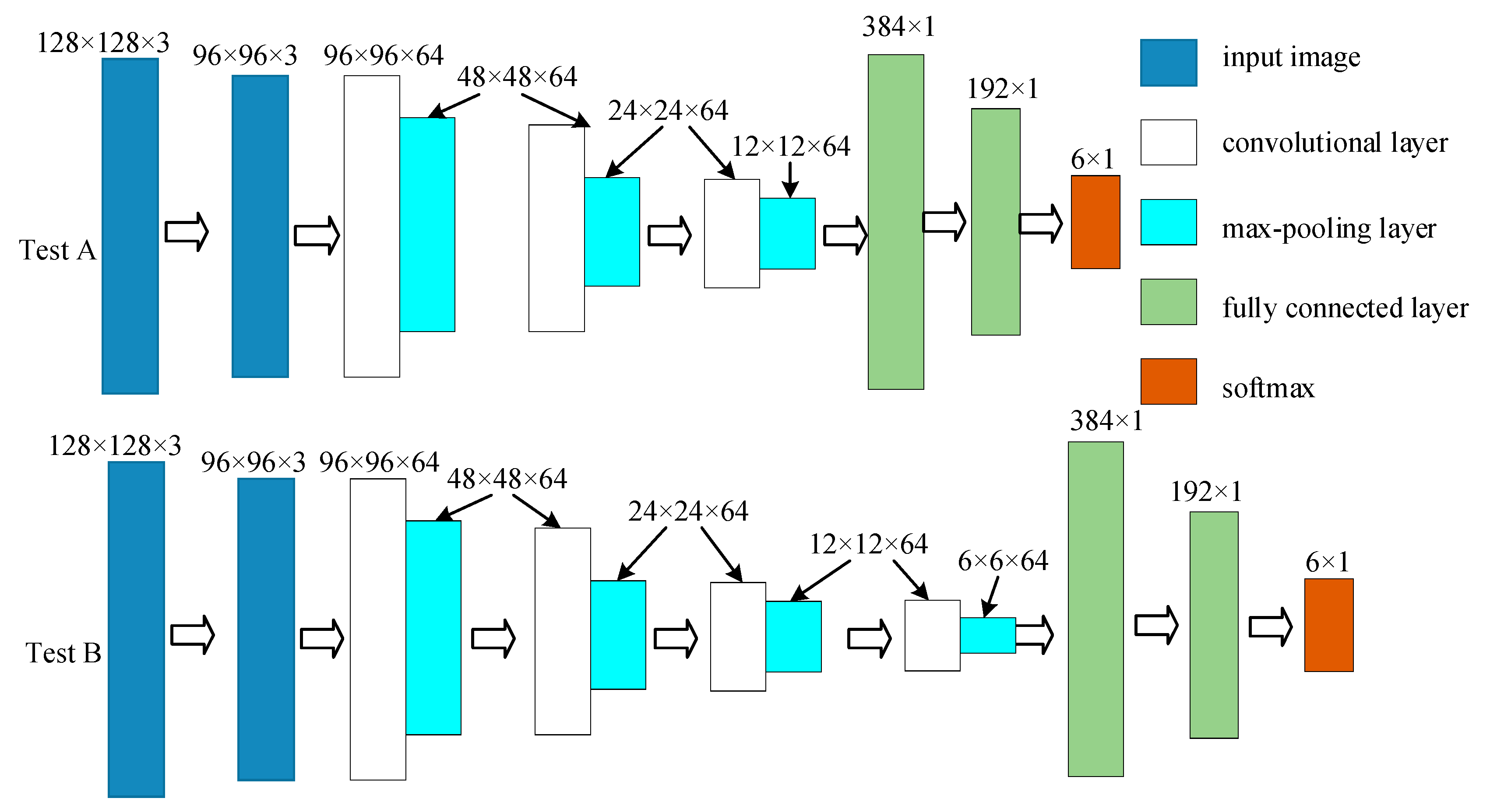
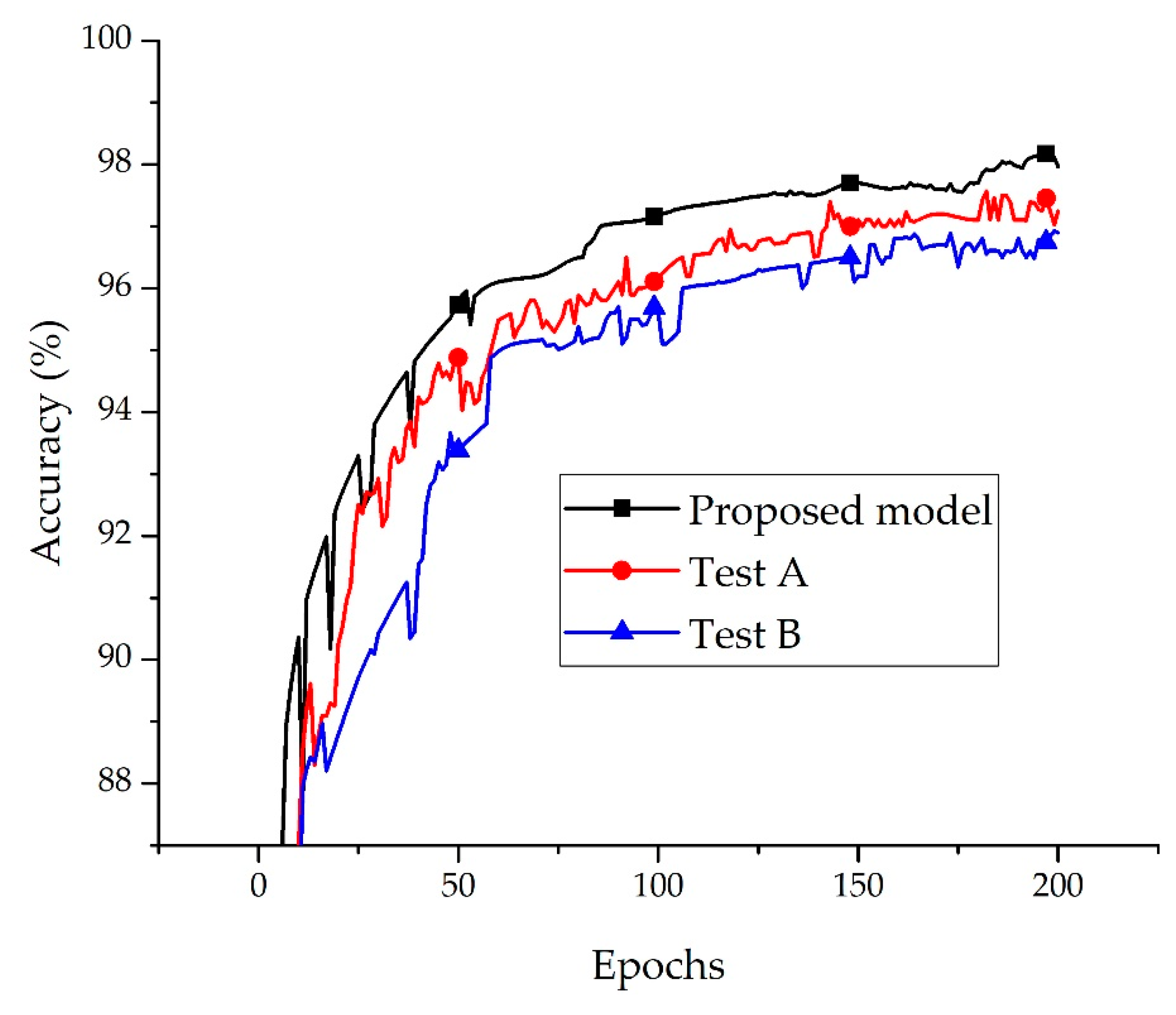
Section 4 analyzes the factors that affect the identification accuracy, such as the type of model, sample size, and model level, and presents the results.
Section 5 provides the conclusions of the study.
2. Architecture of the Rock Types Deep Convolutional Neural Networks Model
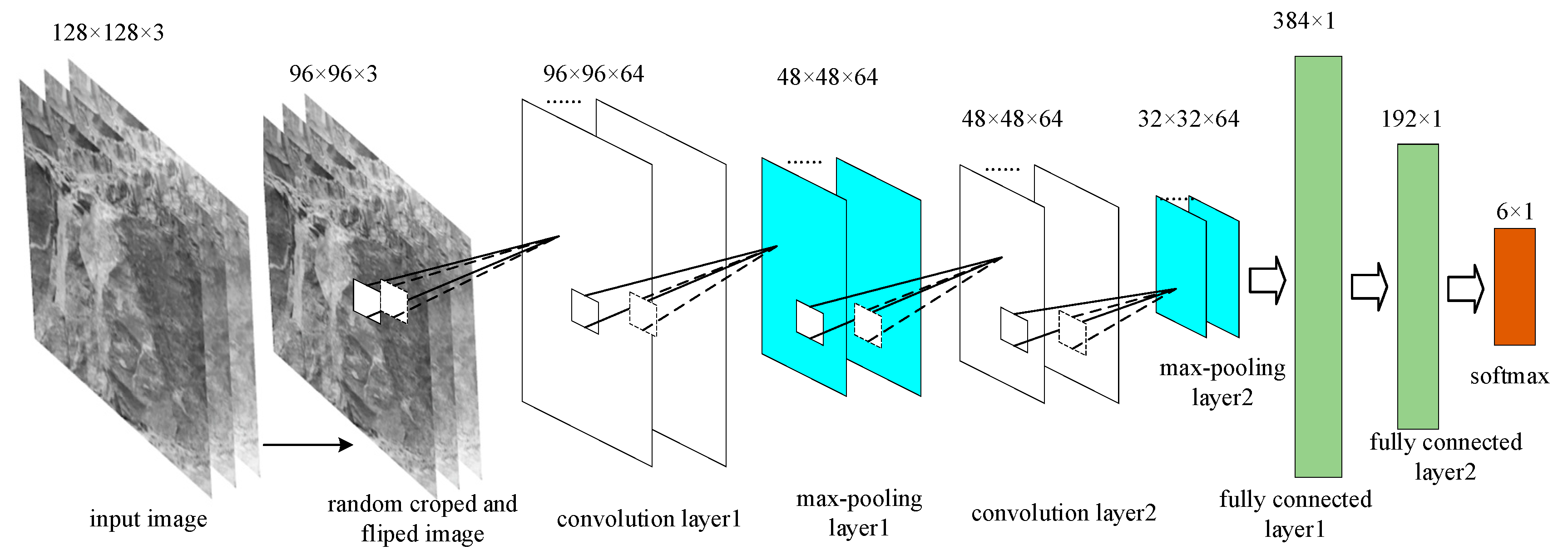
Developments in deep learning technology have allowed continuous improvements to be made in the accuracy of CNNs models. Such advances have been gained by models becoming ever deeper, which has meant that such models demand increased computing resources and time. This paper proposes a RTCNNs model for identifying rock types in the field. The computing time of the RTCNNs model is much less than that of a model 10 or more layers. The hardware requirements are quite modest, with computations being carried out with commonly used device CPUs and Graphics Processing Units (GPUs). The RTCNNs model includes six layers (
Figure 2).
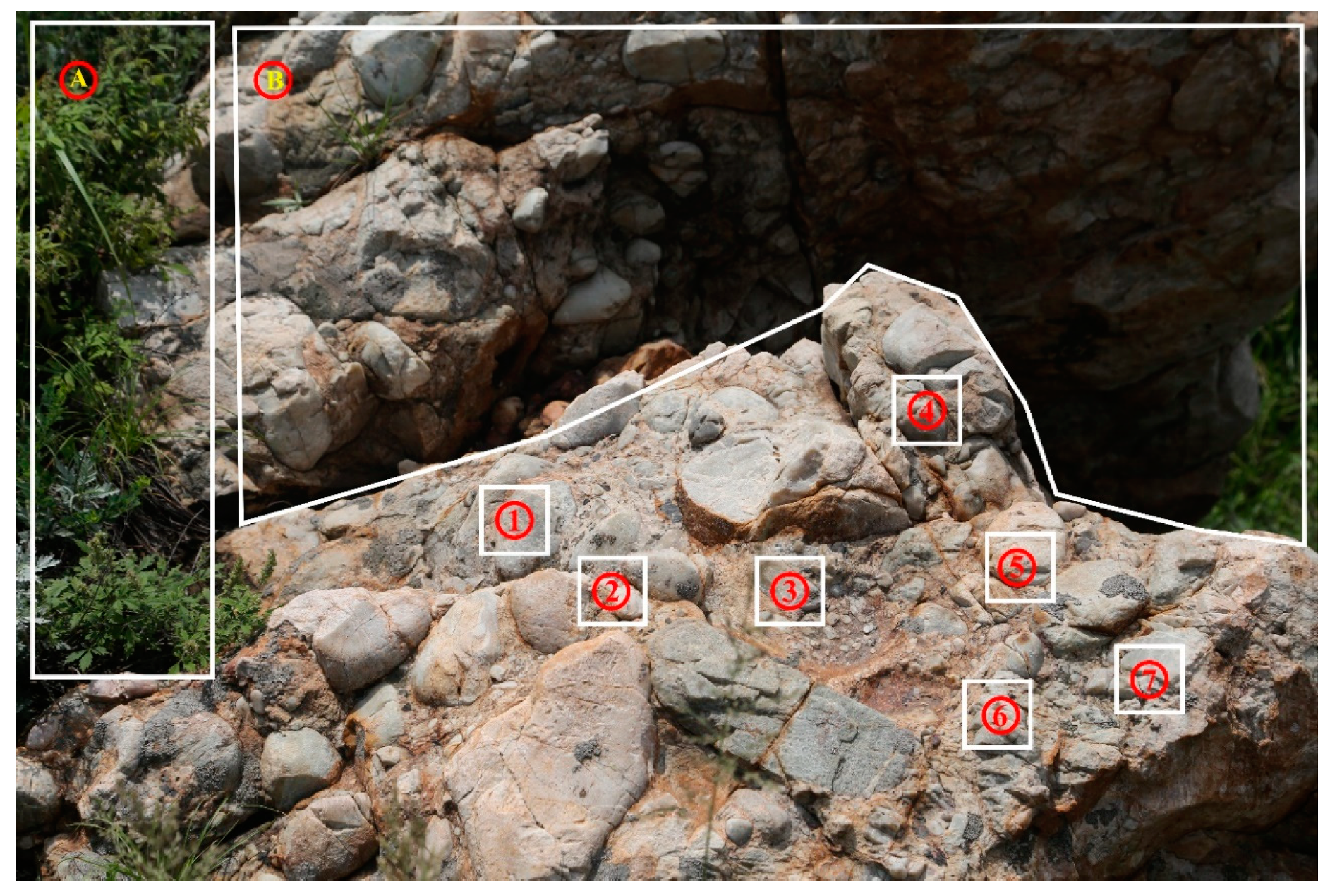
Before feeding the sample images into the model, Random_Clip and Random_Flip operations are applied to the input samples. Each part of the image retains different feature of the target object. Random clipping can reserve the different features of the image. For example, partition A of the image shown in
Figure 1 records smaller changes in grain size of mylonite, in which quartz particles do not undergo obvious deformation, while partition B records larger tensile deformation of quartz particles, and the quartz grains in the partition C are generally larger. In addition, in the proposed model, each layers of training have fixed size parameters, such as the input size of convolution layer1 is 96 × 96 × 3, while the output size of feature is 96 × 96 × 64 (
Figure 2). The input images are cropped into sub-images with given size, while the given size is less. In the proposed model, the cropped size is 96 × 96 × 3, while the input size is 128 × 128 × 3. Through the random clipping operation of fixed size and different positions, different partitions of the same image are fed into the model during different training epochs. The flipping function can flip the image horizontally randomly. Both clipping and flipping operations are realized through the corresponding functions of TensorFlow deep learning framework [
28]. The sample images fed into the model are therefore different in each epoch, which expands the training dataset, improving the accuracy of the model and avoiding overfitting.
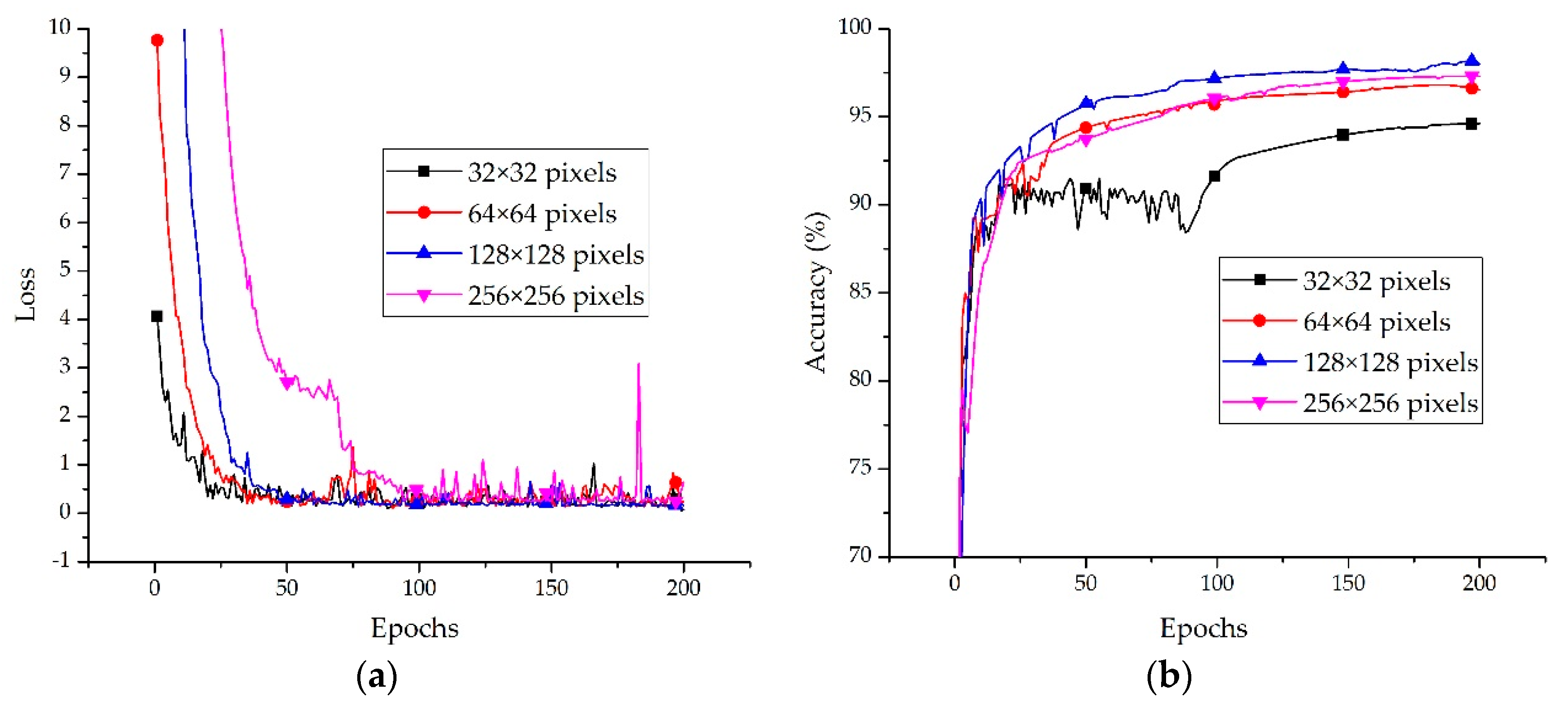
Before performing patch-based sampling, the various features of the rock are spread all over the entire original field-captured image. The experiments described in
Section 4 show that a smaller convolution kernel can filter the rock features better than the bigger kernel of other models. As a consequence, the first convolutional layer is designed to be 64 kernels of size 5 × 5 × 3, followed by a max-pooling layer (
Section 2.2), which can shrink the output feature map by 50%. A Rectified Linear Unit (ReLU,
Section 2.3) activation function is then utilized to activate the output neuron. The second convolutional layer has 64 kernels of size 5 × 5 × 64 connected to the outputs of the ReLU function, and it is similarly followed by a max-pooling layer. Below this layer, two fully connected layers are designed to predict six classes of field rock, and the final layer consists of a six-way Softmax layer. Detailed parameters of the model, as obtained by experimental optimization, are listed in
Table 1.
2.1. Convolution Layer
A convolution layer extracts the features of the input images by convolution and outputs the feature maps (
Figure 3). It is composed of a series of fixed size filters, known as convolution kernels, which are used to perform convolution operations on image data to produce the feature maps [
29]. Generally, the output feature map can be realized by Equation (1):
where
represents the
th layer,
represents the value of the feature, (
i,
j) are coordinates of pixels,
represents the convolution kernel of the current layer, and
is the bias. The parameters of CNNs, such as the bias
and convolution kernel
are usually trained without supervision [
11]. Experiments optimized the convolution kernel size by comparing sizes of 3 × 3, 5 × 5, and 7 × 7; the 5 × 5 size achieves the best classification accuracy. The number of convolution kernels also affects the accuracy rate, so 32, 64, 128, and 256 convolution kernels were experimentally tested here. The highest accuracy is obtained using 64 kernels. Based on these experiments, the RTCNNs model adopts a 5 × 5 size and 64 kernels to output feature maps.
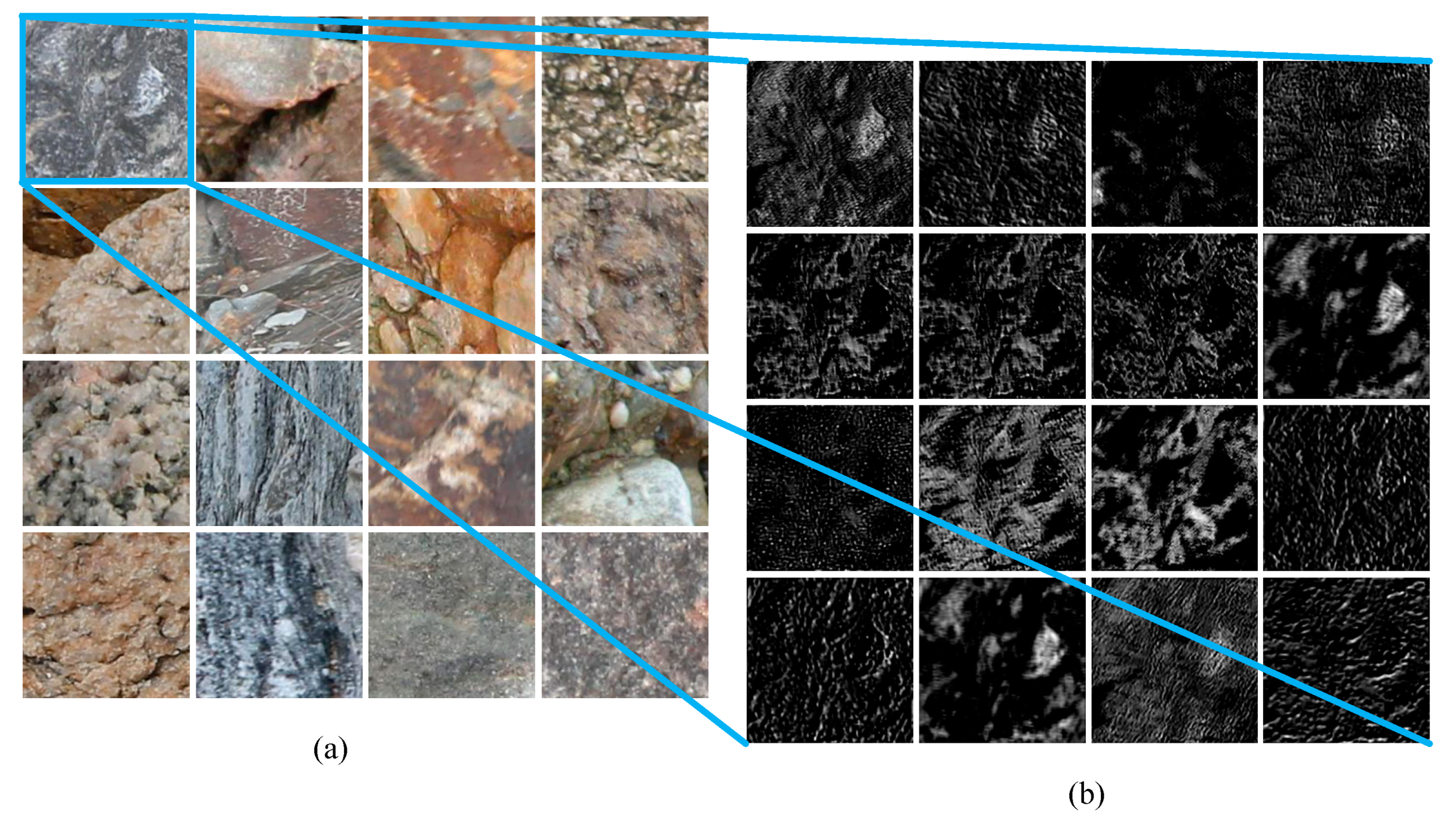
Figure 3 shows the feature maps outputted from the convolution of the patched field images.
Figure 3a depicts the patch images from field photographs inputted to the proposed model during training, and
Figure 3b shows the edge features of the sample patches learned by the model after the first layer convolution. The Figure indicates that the RTCNNs model can automatically extract the basic features of the images for learning.
2.2. Max-Pooling Layer
The pooling layer performs nonlinear down-sampling and reduces the size of the feature map, also accelerating convergence and improving computing performance [
12]. The RTCNNs model uses max-pooling rather than mean-pooling because the former can obtain more textural features than can the latter [
30]. The max-pooling operation maximizes the feature area of a specified size and is formulated by
where
is the pooling region
in feature map
,
is the index of each element within the region, and
is the pooled feature map.
2.3. ReLU Activation Function
The ReLU activation function nonlinearly maps the characteristic graph of the convolution layer output to activate neurons while avoiding overfitting and improving learning ability. This function was originally introduced in the AlexNet model [
14]. The RTCNNs model uses the ReLU activation function (Equation (3)) for the output feature maps of every convolutional layer:
2.4. Fully Connected Layers
Each node of the fully connected layers is connected to all the nodes of the upper layer. The fully connected layers are used to synthesize the features extracted from the image and to transform the two-dimensional feature map into a one-dimensional feature vector [
12]. The fully connected layers map the distributed feature representation to the sample label space. The fully connected operation is formulated by Equation (4):
where
is the index of the output of the fully connected layer;
m,
n, and
d are the width, height, and depth of the feature map outputted from the last layer, respectively;
represents the shared weights; and
is the bias.
Finally, the Softmax layer generates a probability distribution over the six classes using the output from the second fully connected layer as its input. The highest value of the output vector of the Softmax is considered the correct index type for the rock images.
5. Conclusions
The continuing development of CNNs has made them suitable for application in many fields. A deep CNNs model with optimized parameters is proposed here for the accurate identification of rock types from images taken in the field. Novelly, we sliced and patched the original obtained photographic images to increase their suitability for training the model. The sliced samples clearly retain the relevant features of the rock and augment the training dataset. Finally, the proposed deep CNNs model was trained and tested using 24,315 sample rock image patches and achieved an overall accuracy of 97.96%. This accuracy level is higher than those of established models (SVM, AlexNet, VGNet-16, and GoogLeNet Inception v3), thereby signifying that the model represents an advance in the automated identification of rock types in the field. The identification of rock type using a deep CNN is quick and easily applied in the field, making this approach useful for geological surveying and for students of geoscience. Meanwhile, the method of identifying rock types proposed in the paper can be applied to the identification of other textures after retraining the corresponding parameters, such as rock thin section images, sporopollen fossil images and so on.
Although CNNs have helped to identify and classify rock types in the field, some challenges remain. First, the recognition accuracy still needs to be improved. The accuracy of 97.96% achieved using the proposed model meant that 99 images were misidentified in the testing dataset. The model attained relatively low identification accuracy for sandstone and limestone, which is attributed to the small grain size and similar colors of these rocks (
Table 5;
Figure 8). Furthermore, only a narrow range of sample types (six rock types overall) was considered in this study. The three main rock groups (igneous, sedimentary, and metamorphic) can be divided into hundreds of types (and subtypes) according to mineral composition. Therefore, our future work will combine the deep learning model with a knowledge library, containing more rock knowledge and relationships among different rock types, to classify more rock types and improve both the accuracy and the range of rock-type identification in the field. In addition, each field photograph often contains more than one rock type, but the proposed model can classify each image into only one category, stressing the importance of the quality of the original image capture.
Our future work will aim to apply the trained model to field geological surveying using UAVs, which are becoming increasingly important in geological data acquisition and analysis. The geological interpretation of these high-resolution UAV images is currently performed mainly using manual methods, and the workload is enormous. Therefore, the automated identification of rock types will greatly increase the efficiency of large-scale geological mapping in areas with good outcrops. In such areas (e.g., western China), UAVs can collect many high-resolution outcrop images, which could be analyzed using the proposed method to assist in both mapping and geological interpretation while improving efficiency and reducing costs. In order to improve the efficiency of labeling, the feature extraction algorithm [
35] will be studied to automatically extract the advantageous factors in the image. We also plan to apply other deep learning models, such as the state-of-art Mask RCNN [
36], to identify many types of rock in the same image. In addition, we will study various mature optimization algorithms [
37,
38,
39] to improve computing efficiency. These efforts should greatly improve large-scale geological mapping and contribute to the automation of mapping.


