We propose here three relevant instances of said functions: (i) a request shaping function that guarantees a better QoS by controlling the delay experienced by the packets traveling in the constrained network and by reducing packet losses; (ii) a caching function that improves the QoS of the IoT system because it reduces the power consumption of the Client and the number of packets to be transmitted in the IoT network, saving network bandwidth and reducing response time, while guaranteeing information freshness; and, finally, (iii) a compression function that improves QoS by reducing the size of a packet, so that the number of transmitted packets and the overhead of a fragmentation mechanism are reduced. Indeed, if the compressed packet can fit in a network frame, fragmentation is not needed; if, instead, the compressed packet still cannot fit in a network frame, the number of transmitted packets is reduced because its length is smaller than its uncompressed version, and the fragmentation overhead is reduced because fragmentation is defined as a mechanism internal to the compression function.
In the following, we describe each proposed extended function highlighting its objectives and showing its possible implementation.
4.1. Requests-Shaping
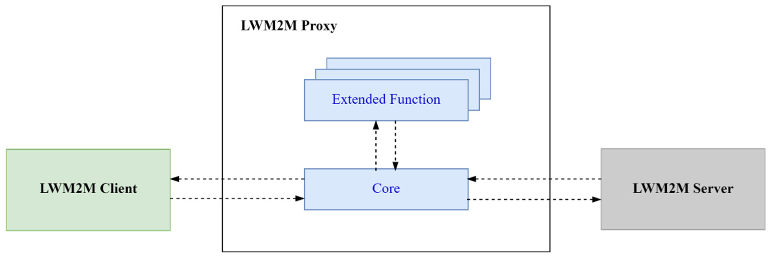
The Proxy can alleviate network congestion by controlling the flow of requests to the Client [
7]; consequently, it can guarantee a better QoS. To do so, the Proxy implements a congestion window that limits the number of outstanding requests over the constrained network up to a fixed maximum. When the Proxy receives a message request for a Client, it enqueues it in a buffer, and forwards it only if the window is open, i.e., if the number of requests forwarded to any Client and still waiting for a response is less than the maximum window size.
4.1.1. Requests Shaping Algorithm
The requests-shaping algorithm behaves similarly to a token-bucket algorithm wherein a token represents a packet. Hence, the bucket is filled with a number of tokens equal to the size of the congestion window. Then, when a packet arrives, it is enqueued in the buffer and, if there is at least one token in the bucket, the Proxy forwards the packet to the Client and it removes one token from the bucket. When the Proxy receives a response to a previous transmitted request, it adds one token to the bucket, checks if a packet is queued for transmission, and possibly transmits it also removing one token from the bucket.
In an extreme case the maximum size of the congestion window is set to one, i.e., there is only one outstanding request. However, in some cases, it can be more efficient to exploit the network resources by sending concurrent requests, i.e., having a maximum congestion window size greater than one. Indeed, the size of the congestion window, i.e., the number of concurrent requests, depends on the number of requests that can be sent through the network without congesting it. This in turn, depends on several factors, including the following: the network/communication technology that is used; the network topology, i.e., the average number of hops to reach the destination; the memory and processing capabilities of the devices, i.e., the size of the buffer used to store incoming packets, and the time needed to process and forward a packet.
4.1.2. Performance Evaluation
To evaluate the advantages of introducing the proposed requests-shaping function, we consider a testbed scenario composed of a sensor network, a Server and a Proxy, as depicted in
Figure 5. A Client runs on a wireless sensor node using the 6LoWPAN protocol [
8] on top of the IEEE 802.15.4 MAC [
19], operating in the 2.4 GHz band, and located three hops away from the 6LoWPAN Border Router. The system is emulated using the COOJA network emulator [
18] and uses RPL [
20] as routing protocol. The Server and the Proxy are developed using the Eclipse Leshan library [
22]. We consider a Client with a sensor that collects information at a periodic sampling rate; indeed, periodic sampling is widely used by IoT devices because the simplicity of periodic sampling is well-fitted with devices which have limited computational resources. The onboard sensor of the Client is a temperature sensor that samples the temperature each 60 s.
We model the arrival of LWM2M requests as a Poisson process with cumulative rate , and we consider the following metrics: (i) service delay, defined as the time between the request is sent by the Server and the time the corresponding response is received, (ii) service loss, defined as the percentage of LWM2M requests that did not receive a response according to requests sent.
First, we evaluate the same scenario considered in
Section 3, now taking into account the case when the Proxy is in place, and we compare the case where the Proxy does not implement the request shaper against the case where the Proxy implements the request shaper with the maximum size of the congestion window fixed to one.
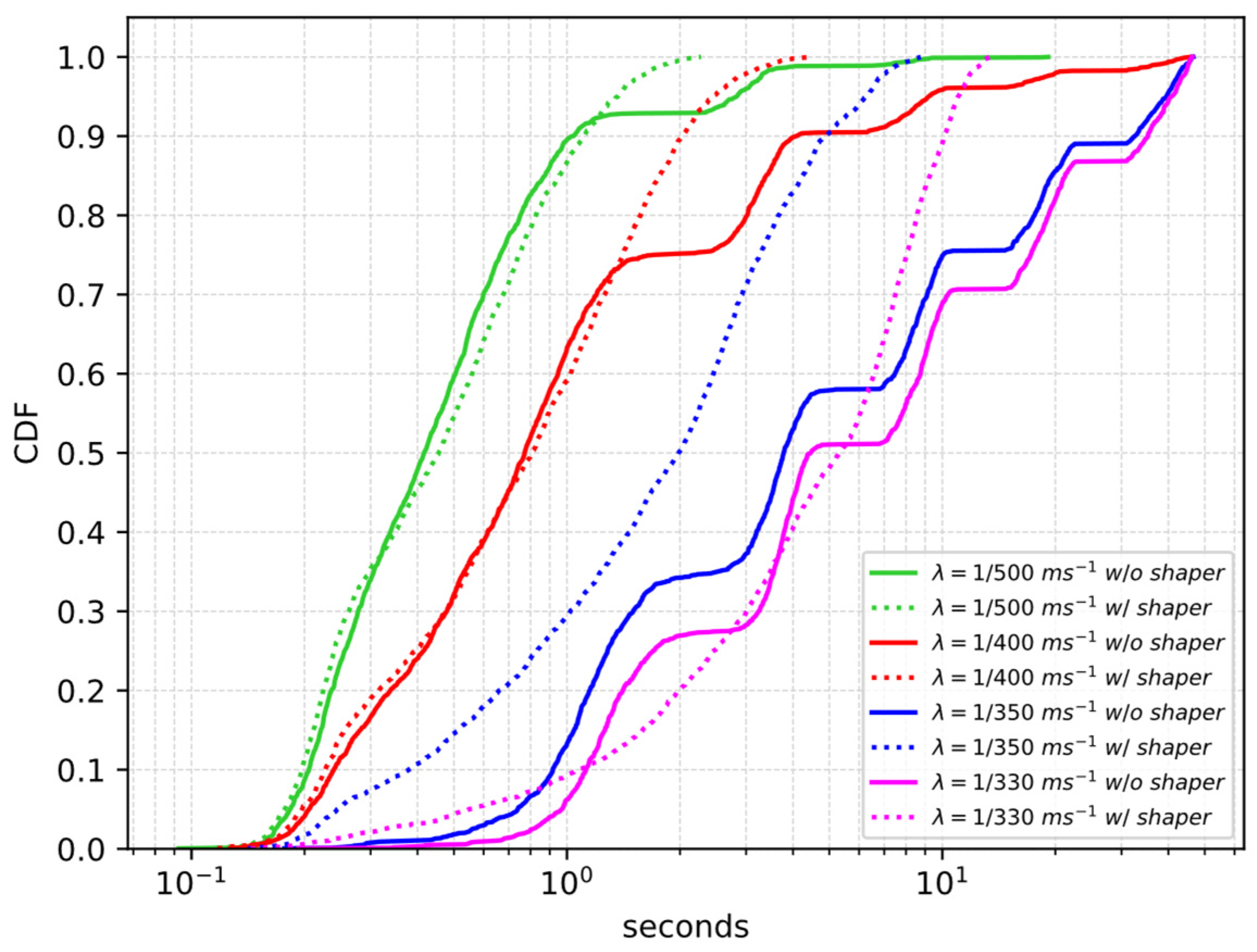
Figure 6 shows the cumulative distribution function of the service delay for different values of
using a log scale on the
x-axis. When the rate
increases, if the Proxy does not implement the request shaper, the distribution shifts to the right and its tail is heavier; in addition to this also the packet loss increases, as reported in
Table 2. Instead, when the request shaper is used, the maximum experienced service delay decreases significantly, the tail of the distribution is shorter and there is no service loss. This happens because the Proxy that uses the requests-shaping function can control the traffic load in the network avoiding congestion. We can notice that the service delay experienced with the requests-shaping function using a window value equal to one is not always better than the service delay experienced without the requests-shaping function. So, a requests-shaping function using a larger window value could perform better.
Figure 7 compares the service delays of the scenarios that use the request shaper against the service delays of the scenarios that do not use the request shaper; the comparison is done using a box plot representation: in the box the 25th, the 50th, and the 75th percentiles are represented, respectively, the ends of the whiskers represent the 5th and 95th percentiles and the circles are the outliers. We can notice that especially for lower values of
i.e., when
= 1/500 ms
−1 or when
= 1/400 ms
−1, the 25th and 50th percentile values obtained with the request shaper and without the request shaper are almost the same; but we can also notice from the 75th and 95th percentile values that with the request shaper the maximum experienced service delay decreases significantly (please note the log scale on the
y-axis).
In the second scenario under consideration, we tested different values for the maximum congestion window size.
Figure 8 shows the cumulative distribution function of the service delay for different values of the congestion window size in the case of a rate
equal to 1/330 ms
−1. We can observe that when the congestion window size is fixed to three the service delay experienced with the request shaper is always better than the service delay experienced without the request shaper. But, of course, when there are concurrent requests in the network it is possible that some of them experience a larger service delay with respect to the case in which there is always only one pending request in the network. Indeed, we can observe that the maximum service delay experienced by the packets in the case of a window value equal to three is larger than the case of a window value equal to one.
4.3. Compression
IoT networks can impose strict limitations on traffic. For example, LPWAN technologies such as LoRaWAN [
10], are characterized by a reduced data rate and a limited payload length in order to support long range and low power operations.
The FUOTA Working Group of the LoRa Alliance addresses this limitation on packet size by defining a fragmentation mechanism. They propose an application layer messaging package [
25] running over LoRaWAN that sends a fragmented block of data to the device. This method splits a data block into multiple fragments to fit into LoRaWAN packets; then, these fragments must be reassembled on the device, handling potential losses. To do so, first a session establishment mechanism must be run to inform the device that a fragmentation session will start. Fragmentation can affect the QoS of the system. Indeed, it introduces overhead because each fragment has to contain the L2 header, and it also introduces delay because a message can be reassembled only after all the fragments have been received. Moreover, LPWAN technologies are characterized by a high packet loss rate, so fragments can be lost causing retransmissions and therefore performance degradation.
We instead propose to reduce the packet size by applying a compression function, thus limiting the need for fragmentation. The compression function is based on the Static Context Header Compression (SCHC, [
26,
27]) framework and executed both on the Client and on the Proxy. SCHC compression relies on a common static context, i.e., a set of rules, stored both in the Proxy and in the Client. The Proxy can define a specific context for each Client to take into account their heterogeneity and the Servers can be unaware of these changes in the communication with the Clients. The Client stores a single context because it exchanges compressed packets only with the Proxy. The context does not change during packet transmission, so SCHC avoids the complexity of a synchronization mechanism. Moreover, SCHC supports fragmentation, thus if the compressed packet size still exceeds the maximum packet size, it is possible to fragment the compressed packet with a reduced overhead and with fewer fragments needed than in the case of the uncompressed packet fragmentation.
The main idea of the SCHC framework is to exploit the fact that the traffic of IoT applications is predictable, so it is possible to transmit the ID of a compression/decompression rule, i.e., rule ID, instead of sending known packet-field values. SCHC classifies fields in (i) static, i.e., well-known, and hence not sent on the link; (ii) dynamic, i.e., sent on the link; (iii) computed, i.e., rebuilt from other information. At the top of
Figure 11 we make an example of a compression/decompression rule: as we can see from the figure, a rule contains a list of field descriptions composed of the following data: (i) Field Identifier (FID), it designates a protocol and a field; (ii) Field Length (FL), it represents the length of the field; (iii) Field Position (FP), it indicates which occurrence of the field this field description applies to; (iv) Direction Indicator (DI), it indicates the packet direction; (v) Target Value (TV), it is the value to match against the packet field; (vi) Matching Operator (MO), it is the operator used to match the field value and the target value; (vii) Compression/Decompression Action (CDA), it describes the compression and decompression actions applied on the field. If the field has a fixed length, then applying the CDA to compress it produces a fixed number of bits, which is called the compression residue of the field. If the CDA is “not sent”, then the compression residue is empty. If, instead, the field has a variable length, e.g., the uri-path or the uri-query, then, applying the CDA may produce either a fixed-size or variable-size compression residue. The former case occurs when the field value is known and hence it is not sent, or when the field value belongs to a known list of values and hence the index of the list is sent. In the latter case, instead, the compression residue is the bits resulting from applying the CDA to the field, preceded by the size of the compression residue itself, encoded as specified in [
27]. If a variable-length field is not present in the packet header being compressed, a size 0 must be specified to indicate its absence. We provide here a brief description of the compression and decompression algorithms of SCHC, whereas in
Section 4.3.1 and
Section 4.3.2. we propose and evaluate an extension to SCHC for LWM2M.
The compression algorithm consists of three steps as follows: (i) rule selection: identify which rule will be used to compress the packet’s headers. The rule will be selected by matching the field descriptions to the packet header; (ii) compression: compress the fields according to the compression actions. The fields are compressed in the order specified by the rule and the compression residue is the concatenation of the residues for each field; (iii) sending: the rule ID is sent followed by the compression residue. The decompression algorithm consists of a single step: (i) decompression: the receiver selects the appropriate rule from the rule ID. Then it applies the decompression actions to reconstruct the original fields.
SCHC allows one to specify a fixed number of fields in a rule. If, instead, a variable number of fields is needed, e.g., when the number of uri-path or uri-query varies, it is possible to either create multiple rules to cover all cases or to create one rule that defines multiple entries and send a compression residue with length zero to indicate that a field is empty. These two options introduce a trade-off between compression ratio and memory usage: indeed, if we define multiple rules that cover all possibilities, we increase the compression ratio, but we also need more memory on the device to store all the rules; if, instead, we define a single rule we obtain a lower compression ratio, but we also need less memory on the device.
To illustrate the SCHC framework, in
Figure 11 we show an example of its possible use in a LWM2M architecture instantiated in a LoRaWAN network: on the left, we show the original uncompressed packet, while, on the right, we show the packet compressed using the rule listed at the top of the figure. Due to the limited bandwidth of LoRaWAN, the LWM2M standard defines the possibility of using CoAP over LoRaWAN (LoRaWAN binding, [
5]) by placing the CoAP packet containing the LWM2M message directly in the LoRaWAN packet payload. Thus, in this case, a set of compression rules for the CoAP header can be defined according to the following criteria:
The CoAP version, type, and token length fields have been elided, since their values are known.
The CoAP code field has been reduced to the set of the used codes for each operation, defining a mapping list.
The CoAP message id has been reduced to a four bits value, using the MSB (most significant bits) matching operator.
The CoAP token field needs to be transmitted, but, since the token length is known, it is not necessary to send the size.
The CoAP content format and accept fields have been elided when only a single value is possible; otherwise, they have been reduced to the set of used values using a mapping list.
The CoAP uri path fields have been elided when only a single value is possible; otherwise, they have been reduced to the set of used values using a mapping list. Since the number of uri path elements may vary, it has been decided to define the length to variable and send a compression residue with a length of 0 when the uri path is empty.
The CoAP uri query fields are used for setting the attributes, so they have been reduced to only their numeric values using the MSB matching operator. Since the number of uri query elements may vary, it has been decided to define the length to variable and send a compression residue with a length of 0 when the uri query is empty.
In the example of
Figure 11, the receiver reconstructs the CoAP version, type, token length, code, and content format using the values stored in the corresponding target value entries; it rebuilds the message id value concatenating the most significant bits stored in the target value entry and the received bits, and it builds the token value from the received value. We can notice that SCHC reduces the size of the packet, from 8 bytes to 12 bits; however, the overall packet-size reduction is limited because the largest component of the packet, i.e., the payload, is still sent uncompressed. We can also notice that the payload marker used to indicate the end of options and the start of the payload is not present in the compressed packet because the length of the compression residue of the header is known; moreover, even if the compression is bitwise, the final size of the compressed packet is byte aligned to be sent on the network.
We refer the reader to [
26,
27,
28] for further details on SCHC.
4.3.1. Extended SCHC for LWM2M
SCHC provides only header compression, so in the previous example the LWM2M payload must be sent uncompressed after the SCHC compression residue. In constrained technologies such as LoRaWAN, the header compression alone might not be enough to fit the maximum allowed packet size. In this work we thus extend the SCHC mechanism to also provide payload compression of LWM2M messages.
The LWM2M message structure can be efficiently compressed using the SCHC mechanism. In fact, a LWM2M Object Instance can be represented by an array of entries where each entry is a Resource, i.e., a ResourceID and its corresponding value, as, for example, a sensor-measurement value. The ResourceID can be considered equivalent to the SCHC FID and, hence, we can straightforwardly apply the SCHC compression algorithm also to the Resource field. When the value of the Resource is dynamic, it is also possible to compress it using a standard data compression algorithm; in this work, we just apply the SCHC compression mechanism.
If a LWM2M message contains multiple Instances of a given Object, the compression/decompression is applied for each Object Instance; the number of Object Instances present in the message is sent before the compression residue using the size encoding [
27]. In more detail, the Object Instances and their Resources are ordered according to their IDs, so that it is possible to either: (i) elide the value of a Resource when it is known a priori, (ii) define a mapping list for a Resource when its value belongs to a defined set of elements, (iii) send the value of the Resource in all the other cases. Instead, when Read/Write operations involve one single Resource, the value of the Resource is sent uncompressed after the CoAP compressed header.
As illustrated in
Section 3, whenever a Client connects to the network, the Proxy retrieves and stores its Objects and, for each of them, the list of supported Resources. We assume that this list does not change during the transaction between the Client and the Proxy. After collecting the supported Resources, the Proxy can create the rules needed for the compression of the messages. In the Client, these rules are represented as LWM2M Objects, so the Proxy can write the context in the Client using LWM2M Write requests. As soon as this initialization phase has been completed, the Proxy and the Client can start exchanging compressed messages.
In
Figure 12 we consider the same example of
Figure 11, now applying the proposed extended SCHC framework. In the figure, the additional field descriptions of the rule that allow the compression/decompression of the LWM2M message are highlighted in red. The compression residue of the CoAP header is the same as that obtained in the example of
Figure 11, now preceded by the number of Object Instances present in the message, i.e., 1, and followed by the compression residue of the LWM2M payload. The LWM2M field descriptions of the rule specify that the Instance ID of the Object has a variable length and its value is sent; in the example, the Instance ID is not present in the LWM2M payload because the request is for a specific Instance of the Object, i.e., for the Instance 0, and not for the Object, so a compression residue with a length of 0 is sent; the value of the Sensor Value Resource is sent; the Sensor Units Resource can take only the three values listed in the TV, so the index of the value in the target value list is sent. We can notice that the packet size is further reduced because the LWM2M message is also compressed.
4.3.2. Performance Evaluation
To illustrate the benefits of introducing a Proxy that implements the compression function, motivated by the payload size issues illustrated in
Section 3, we instantiated the proposed architecture in a LoRaWAN network [
10].
To cope with such constrained underlying technology, we implemented the LoRaWAN binding in addition to the compression function. We assume that the device that runs the Client implements only the LWM2M application, so the communication is end-to-end with the Proxy and the IP and UDP layers becoming overhead and able to be easily removed. As a consequence, the packet size is reduced and the number of computations and exchanged messages are reduced as well, because the Client does not have to manage the IP protocol stack.
The packet size is further reduced by applying the proposed compression mechanism based on the SCHC framework both on the Client and on the Proxy.
We implement a simple LoRaWAN system architecture composed of (see
Figure 13):
a Client. The device that runs the Client is an Heltec WIFI LoRa 32 (V2) and implements a Server Object Instance (ObjectID: 1), a Device Object Instance (ObjectID: 3), and a Temperature Object Instance (ObjectID: 3303). Each of these Objects implements the mandatory resources. The Read, Write, and Execute operations are implemented for Server and Device Objects. The Observe, Notify, and Cancel Observation are implemented for Temperature Object.
a LoRaWAN Gateway. The gateway is a Laird Sentrius RG186. The gateway relays messages between devices and a network server in the backend using the Gateway Message Protocol (GWMP) [
29]. Thus, communication between gateways and network server is via JSON/GWMP/UDP/IP.
a LoRaWAN Network Server. The network server routes the packets to the application server.
a LWM2M Proxy/LoRaWAN Application Server. The communication between the application server and the network server is via JSON over TCP over IP [
30].
a Server.
All the servers are Java servers and the Proxy and the Server use the Eclipse Leshan library [
22] to implement the LWM2M protocol.
Table 3 shows compression results. Compression is applied both to Object Instances, i.e., when reading the Device Object Instance, the Server Object Instance, and the Temperature Object Instance, and when writing the Server Object Instance, and to Resources or to a set of Resources, i.e., when reading a single Resource of the Device or Server Object Instance and when writing one or more Resources of the Server Object Instance. When considering operations involving Resources, we obtain different compression ratios depending on the number of bytes used to represent the resource itself, e.g., the Lifetime Resource (ID: 1) of the Server Object is an integer, while the Binding Resource (ID: 7) of the Server Object is a string.
The compression function is effective because the size of the compressed packet is always smaller than that of the uncompressed one. This compression function can greatly reduce the packet size, especially when it conveys an Object Instance or an Object; indeed, from
Table 3 we can observe that the maximum percentage reduction of the packet is 75% and is obtained when considering the response to a Read request for the Server Object Instance of the Client; and the mean percentage reduction of packets containing an Object Instance is 58.6%. However, the compression function can bring remarkable benefits also when the packets convey just one or more Resources: results show that for these packets the mean percentage reduction is 46.1%. Moreover, the compressed message always fits in a LoRaWAN packet.


