1. Introducción
Snow is a defining regulator of the global energy budget and ecosystem function, governing both ecologic and hydrologic responses to climate variability. Warming across the high latitudes in the Northern Hemisphere has contributed to reduced snow cover [
1], whereby the reduced surface albedo from less snow cover [
2,
3] enhances the solar energy loading that promotes additional thawing that reinforces further climate warming [
1,
4,
5,
6]. In Alaska, the snow-free season has lengthened, prompting a cascade of environmental impacts [
3], including earlier onset of snowmelt and seasonal flooding in spring; earlier and longer potential growing seasons [
7,
8]; changes in permafrost active layer conditions, vegetation growth, and ecosystem net carbon uptake [
9,
10]; and reductions in plant diversity [
11,
12]. Quantifying the spatial and temporal trends in regional snow cover changes is important for better understanding the regional impacts of a warming climate on boreal-Arctic ecosystems.
Snow cover assessments can be obtained from models, in situ observations, remote sensing, or a combination of these. In Alaska, snow has been modeled using climate data products including the Parameter Elevation Relationships on Independent Slope Model (PRISM) and the Modern-Era Retrospective analysis for Research and Applications (MERRA-2) [
13,
14]. These products are often limited by coarse spatial resolution (1–50 km) and/or limited spatial coverage. The Alaska Snow Telemetry (SNOTEL) network provides high quality in situ snow measurements of depth, density, and snow water equivalent (SWE); however, the utility of these measurements is limited by a very sparse station distribution in northern, boreal-arctic ecosystems that is inadequate to represent landscape heterogeneity and snow redistribution mechanisms [
1,
15,
16,
17]. Remote sensing offers a remedy to the limitations of both modelled and in situ snow observations for regional assessment and monitoring of snow conditions. A variety of satellite platforms and sensor types have been used for the remote sensing of snow, including passive optical-infrared sensors [30–500 m], Lidar [~1 m], microwave Radars and scatterometers [25 km], and passive microwave radiometers [25 km]. Each sensor type is sensitive to different snow properties, while providing variable sampling footprints, accuracy, and spatial and temporal coverage.
Snow properties derived from remote sensing observations include: snow covered area [
18,
19,
20], snow depth [
21,
22], SWE [
23], main melt onset [
24,
25], and snow wetness [
26]. Determining the date of snowoff (SO)—defined here as the last day of observed seasonal snow cover in spring—is particularly valuable from an ecosystem perspective because it is tractable and is a key metric influencing other environmental variables, including: the start of spring carbon uptake, snowmelt duration [
8,
27], wildlife ecology and movement [
17], and the timing of hydrologic events [
28]. SO has been defined using several terms, including but not limited to: snow disappearance [
29], snow clearance day [
9], melt-off day [
30], and snow persistence [
31]. Optical remote sensing methods have generally determined SO using a threshold value of single channel spectral reflectance data or channel combinations such as the Normalized Difference Snow Index (NDSI) [
32].
Relatively high-quality SO data products with spatial projections for Alaska include the Alaskan MODIS Snow Cover Metrics and Landsat Snow Persistence Maps. The Alaskan Snow Cover Metrics are a suite of complimentary snow parameters derived from the Moderate Resolution Imaging Spectrometer (MODIS) at 500 m spatial resolution, with SO defined as the last day of the longest continuous snow season (LCLD) [
13]. The annual Alaskan Landsat Snow Persistence Maps represent the last day snow persisted, and have a native 30 m spatial resolution and observational record that extends from 2001 to present [
31]. Despite the good overall quality of these products, there is inherent uncertainty introduced from infrequent image acquisition intervals (i.e., 16-day for Landsat) and coarse temporal compositing of the optical-infrared sensor retrievals required to mitigate contaminating effects from clouds and atmosphere aerosols, low solar illumination at higher latitudes (≥45°N), and the inherent errors associated with optical remote sensing of snow [
33]. Furthermore, both the MODIS and available Landsat snow products have a temporal record beginning in 2001, making it difficult to evaluate longer-term trends and variability.
Satellite passive microwave (PMW) sensors offer several advantages over optical sensors because they provide global daily coverage and are insensitive to potential signal degradation from low solar illumination and atmosphere cloud-aerosol contamination [
34]. Furthermore, PMW sensors, including the Defense Meteorological Satellite Program (DMSP) Special Sensor Microwave Imager (SSM/I) (1987–present) and Special Sensor Microwave Imager/Sounder (SSMIS) (2004–present), are sensitive to snow cover properties and provide continuous global observations from similar overlapping satellites extending as far back as 1987. SO has been calculated from PMW retrievals using several approaches, including snow cover duration (SCD) [
9], spring thaw timing [
35,
36], wavelet transformations of brightness temperature (Tb) time series [
27], Tb diurnal amplitude variations (DAV) [
37,
38], and Tb differencing algorithms [
30,
39]. A common physical basis for snow retrieval among these methods is the differential response in microwave emissions at 19 (V, H) GHz and 37 (V, H) GHz frequencies to changes in liquid water content of the surface snowpack.
Optical and PMW sensors both have limitations for effective snow retrievals. Variable snow cover reflectance properties in complex terrain, overlying vegetation cover, unfavorable lighting, and persistent cloud-atmosphere aerosol contamination can severely constrain optical remote sensing of snow cover in the boreal-Arctic. While many of these limitations are reduced or minimized from PMW remote sensing, the microwave snow retrievals are affected by other constraints including a relatively coarse sampling footprint required to achieve an adequate signal-to-noise ratio, and the contaminating influence of open water, underlying soil, and dense vegetation within the sensor footprint. The resulting satellite snow products can show inconsistent results even for the same snow metrics because of the differences in the underlying sensor characteristics and retrieval algorithms [
13]. In this study, we developed a new satellite SO record for Alaska using PMW daily 19V (K-band) and 37V (Ka-band) GHz Tb observations extending from 1988–2016. We used a spatially enhanced Special Sensor Microwave Imager Sounder (SSM/I(S)) Tb record for the SO retrievals, with four-fold (6.25 km resolution) improved spatial gridding for delineating regional snow patterns relative to the SSM/I(S) native footprint retrievals [25 km]. The PMW SO record is validated against in situ snow depth observations from regional weather stations and compared with other available regional SO records derived from MODIS, Landsat, and model-based assessments. The objectives of this study are to: (i) elucidate the roles of fractional water inundation, forest cover, and topographic complexity as sources of uncertainty as compared to in situ observations and other remote sensing SO products; and (ii) investigate recent SO regional trends enabled from a longer (29-year) satellite PMW record. A major premise for this study is that the satellite PMW record provides daily temporal fidelity and moderate spatial resolution, enabling better SO accuracy and performance relative to other available SO records from satellite optical remote sensing.
2. Study Area and Materials
Alaska spans a large area, approximately 20° of latitude and 50° of longitude, encompassing the North Pacific, Arctic Boreal, and Arctic Ocean regions of the extratropical (>50°N) Northern Hemisphere. Within this region, multiple gradients influence the climate, including latitude, distance from large water bodies, the relative thermal mass and circulation of coastal waters, the location and orientation of major mountain ranges, and elevation. With over 10,000 km of coastline, the region is bounded by the Pacific Ocean to the south and the shallower, seasonally ice-covered Bering, Chukchi and Beaufort seas to the west and north that provide sources of moisture and thermal gradients that drive seasonal weather. This high latitude region also plays an important role in the earth’s energy, water and carbon cycles, and is highly vulnerable to recent climate warming [
3,
40]. Much of the region is snow covered for 6 to 9 months of each year; thus snow is an integral component of the ecosystem and a phase change from snow to rain has potentially profound implications for ecosystem structure and function. Thirteen climate divisions have been described for the state of Alaska [
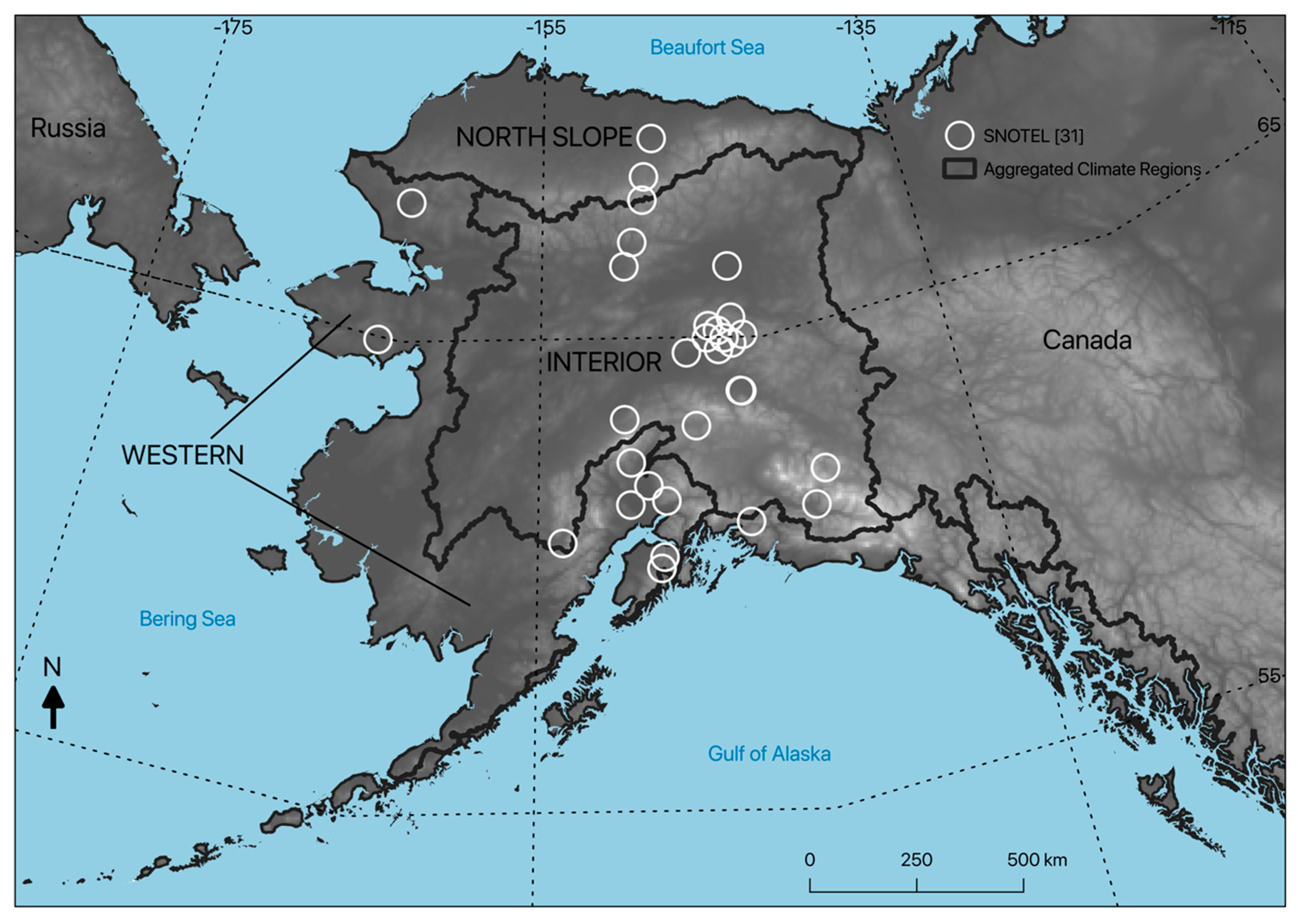
41], which we aggregated into three broader regions for the spatial SO analysis, including Interior, Western and North Slope domains (
Figure 1). These domains reflect Alaska’s major climatic regimes representing moderate Pacific maritime, cold-dry boreal interior, and polar arctic northwest coast and North Slope climate zones. The spatial extent of the PMW-derived SO record from this study includes Alaska, the Russian Far East, and northwest Canada (See
Supplementary materials); however, our comparative analysis covers a smaller domain defined by the Landsat snow persistence product [
31].
2.1. Passive Microwave Record 1988–2016
We detected SO using the SSM/I(S) 19 and 37 GHz ascending orbit (~17:00 local solar time) Tb retrievals at horizontal (H) and vertical (V) polarizations from the MEaSUREs Calibrated Enhanced-Resolution Passive Microwave Daily EASE-Grid 2.0 Brightness Temperature ESDR, available at the National Snow and Ice Data Center (NSIDC) [
42]. This data record is a temporally extensive consortium of images from multiple sensors and platforms. The spatial resolution of the 19 and 37 GHz Tb channels used in this study are improved from the original 25-km resolution Tb format through spatially enhanced interpolation of overlapping Tb antenna patterns and regridding at 6.25 km (19 GHz) and 3.125 km (37 GHz) resolution in a northern polar EASE-grid format using the scatterometer image reconstruction (SIR) technique [
43].
The SSM/I(S) Tb retrievals from different DMSP satellite platforms are highly correlated and only small improvements are made using correction techniques [
44], allowing us to use overlapping observations from the DMSP F-series satellites during the SSM/I and SSMIS era to gap-fill missing coincident grid cells using a nearest-neighbor substitution. Any remaining missing days were gap-filled using a temporal linear interpolation [
25]. The gap-filled daily Tb retrievals were clipped and reprojected to the Alaska Albers Conical Equal Area Projection using the North American Datum 1983 to match the same spatial extent and projection as the MODIS derived snow metrics for Alaska [
13].
2.2. Deriving SO
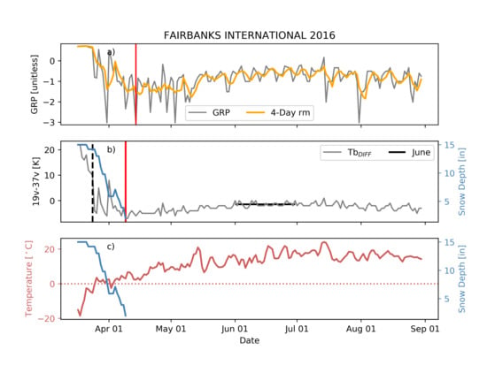
We use the 19V–37V Tb differencing as the primary approach to detect SO [
45], defined here as the last day of snow cover in spring. The resulting Tb difference is strongly positive and relatively stable prior to the seasonal onset of snowmelt indicated from in situ weather station observations (
Figure 2). However, once the snow begins to melt the Tb difference between the two channels precipitously decreases, mirroring the snow ablation rate before reaching a seasonal minimum and becoming more temporally stable following snowoff and moving into the summer. The Tb difference reaches a seasonal minimum just after the snow has finished ablating, which we use to represent the SO condition. We observe a larger positive Tb difference between 19V and 37V GHz channels under colder winter temperatures because the emissivity is greatest at 19V relative to 37V in dry snow conditions. The Tb frequency difference is minimized as snow depth decreases and the liquid water content of the snowpack increases. Shortly after snowpack depletion the land surface is relatively wet and the microwave emissivity is generally larger at 37V than 19V GHz [
46,
47]; hence we define SO as the date when the 19V and 37V difference is at its lowest.
We use a dynamic Tb differencing approach by first calculating the average annual Tb difference value (
sum) for June, which is used as a threshold to identify possible SO dates. We then classify the SO date where the daily Tb difference is less than
sum and has the lowest value of all other potential selections (
Figure 2). We found that the Tb differencing approach was unable to provide reliable SO detection in coastal grid cells, which was attributed to greater water body contamination of the Tb retrievals over adjacent land areas [
48]. The affected grid cells represent 2–3% of the study domain per year. For these instances we used an alternative gradient ratio polarization (GRP) algorithm [
26,
49] to detect SO. For the GRP approach, SO was classified for each grid cell as the day with lowest 4-day running GRP mean (rm) over each seasonal cycle (January–July).
2.3. Gridded SO Datasets
In addition to validating the PMW SO dates against SNOTEL measurements, we also compare the PMW SO with other satellite-derived Alaskan SO dates. The comparisons are quantified as residuals (days) showing the location and magnitude of PMW SO occurring earlier or later relative to the other SO records.
2.3.1. Alaskan Snow Metrics from MODIS
The Alaskan Snow Metrics cover Alaska, northwestern Canada, and the Russian Far East. The data originate from the MODIS Terra Snow Cover Daily L3 Global 500 m Grid data (MOD10A1) [
50] from 2001–2016. The data are provided annually as 12 band GeoTIFFs—each band representing a different snow cover metric. The MODIS MOD10A1 product is a binary snow cover extent dataset derived from the NDSI. Data processing involves a 3-step filtering process to fill the data gaps, including a spatial and temporal filter, as well as a snow cycle filter [
13]. In this study, we used the last day of continuous snow cover (LCLD) to represent SO and resampled each GeoTIFF image using the median LCLD value to match the same 6.25 km resolution and dimensions as the PMW-derived SO record.
2.3.2. Alaskan Snow Persistence
Snow persistence is defined as the transition from snow to snow-free surface conditions. The Alaskan annual snow persistence maps begin in 2001 and are roughly constrained to the Alaskan state boundaries [
31]. This dataset is derived from Landsat (TM, ETM+, OLI) observations and provides a relatively high-resolution (30 m) estimation of annual SO across Alaska. After shadows and clouds are filtered from the 16-day Landsat optical reflectance data, daily snow cover extent is calculated using the NDSI. The remaining unmasked NDSI time series is then used in a regression tree model to predict SO in days of year (DOY) for each 30m grid cell [
31]. The Landsat 30 m Alaska SO record used in this study extended from 2001–2017 and was resampled using the median value and returned the same 6.25 km grid projection as the PMW SO record. We also assigned a minimum +/−16 day precision threshold to the Landsat SO record based on the Landsat 16-day potential sampling frequency, which was used to assess the relative performance of the PMW SO record developed from this study.
2.3.3. IMS
The Interactive Multisensor Snow and Ice Mapping System (IMS) daily snow cover extent record covers different years and spatial grid formats, including 1 km (2014–present), 4 km (2004–present), and 24 km (1997–present) resolutions across the Northern Hemisphere. The IMS snow data are derived using expert interpretation of geostationary visible satellite imagery, polar orbiting multispectral satellite sensors, PMW sensors, and ground observations [
51,
52]. The IMS daily snow cover extent is one of the highest performing snow cover products available, likely attributed to its use of a trained analyst in combination with automated classifications and inclusion of ground observations, which decrease the influence of clouds [
53]. In this study, we used the 4 km IMS snow cover extent product and calculated SO as the first day of 14 consecutive days of snow free conditions for each grid cell [
30]. We assigned a +/−14 day precision threshold to the IMS derived SO record based on the 14-day moving window classification, which was used as a basis for evaluating our PMW SO record. The IMS data were also resampled to the same PMW 6.25 km resolution format using the median value. A summary of each satellite SO dataset used in this study is given in
Table 1.
2.4. Ancillary Datasets
In situ snow depth observations were used to validate the PMW SO algorithm and compare uncertainty between each SO dataset. Like the IMS SO, we defined in situ SO as the first day of 14 consecutive days where snow depth was zero. We used snow depth observations from 31 SNOTEL stations across Alaska and constrained our validation and comparison period to 2004–2016, the common period that all gridded SO datasets share.
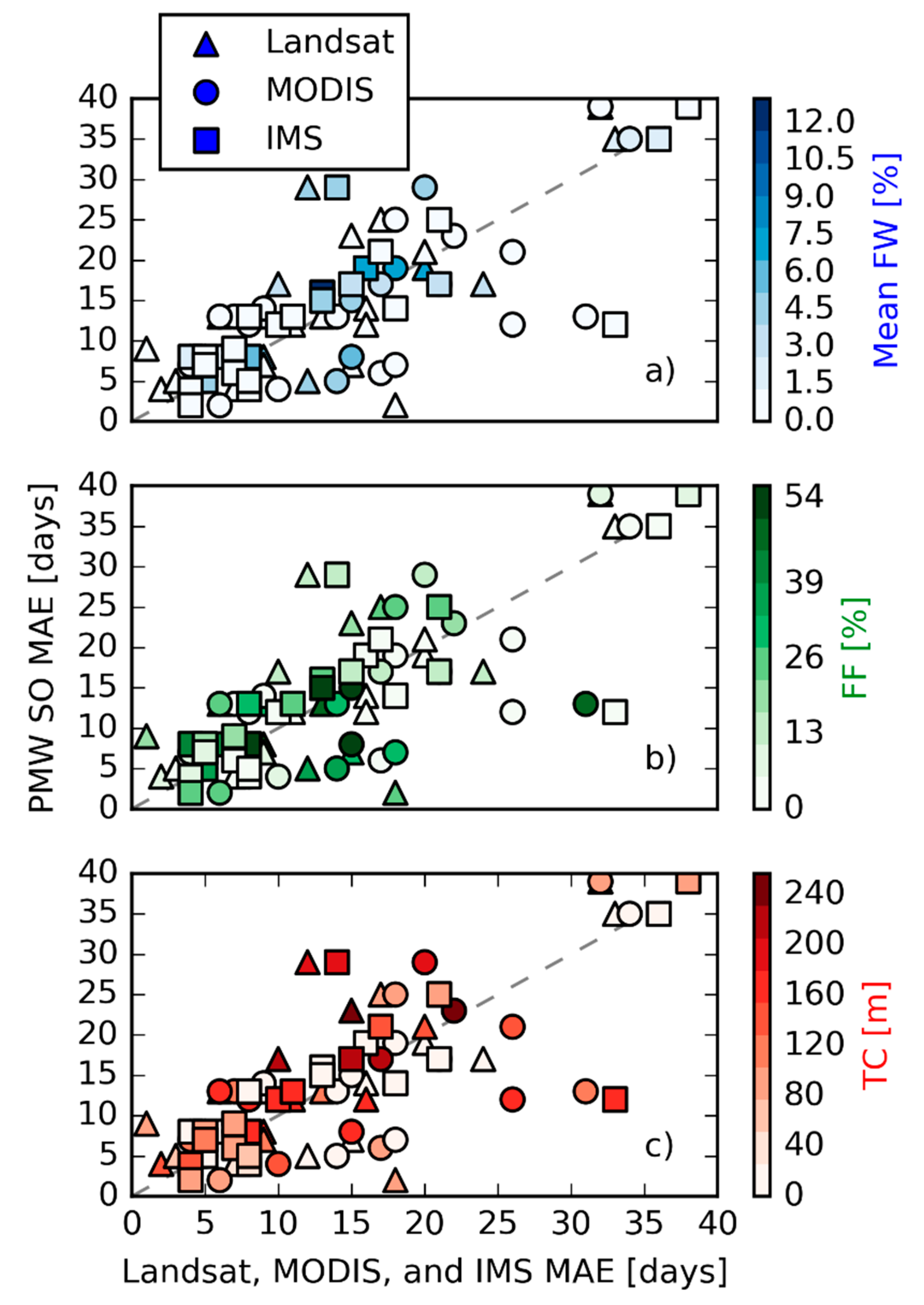
We examined the influence of three land surface properties potentially influencing the PMW SO accuracy, including surface fractional water inundation (FW), fractional forest cover (FF), and the elevation gradient within a grid cell [
54,
55]. We used the dynamic 5-km FW record derived from the Advanced Microwave Scanning Radiometer sensors (AMSR-E and AMSR2), calculated as 10-day FW outputs [
56]; the FW record used here is derived from higher frequency (89 GHz) Tb retrievals than the PMW SO record, but has similar spatial resolution and microwave sensitivity to surface water. We calculated the annual mean FW cover during the summer months from 2002 to 2015 for each grid cell. The PMW performance was then evaluated along a regional gradient in surface water conditions based on the FW summer mean and coefficient of variation (CV) (
Figure 3). Grid cells with significant open water cover (FW > 5 %) were masked from the SO validation to reduce the effect of surface water contamination of the Tb retrievals [
57]. We also excluded grid cells where the FW exceeded a 70% CV threshold, indicating areas with large summer inundation variability. The total area excluded by the FW screening represented approximately 14% of the study domain (
Figure 3c). We also masked out perennial snow/ice areas identified in the Landsat snow persistence images, which represented an additional of the Alaska domain.
The MODIS MOD44B V005 Vegetation Continuous Fields (VCF) product was used to represent the percent tree cover (FF) within each 6.25 km SO grid cell, as defined from the MODIS 250 m native VCF pixel resolution. The VCF has an estimated error of +/−11.5% and is acceptable for our applications [
58]. We also used the GTOPO30 digital elevation model (DEM) with 1 km native resolution to calculate the topographic complexity (TC) within each 6.25 km SO grid cell; where TC was calculated as the spatial standard deviation of the elevation within a cell.
2.5. Assessing the Performance of the PMW SO Algorithm
2.5.1. SNOTEL Validation
The PMW SO results were validated against SO estimates derived from in situ daily weather station observations from Alaska NRCS SNOTEL sites (
Table A1). The mean absolute error (MAE) was derived between each SNOTEL site based SO estimate and the satellite SO retrieval from the overlying PMW grid cell for each site location. Similar MAE metrics were also calculated for the MODIS, Landsat, and IMS SO datasets at each SNOTEL location. The MAE results were then used to evaluate PMW SO accuracy and performance relative to the other SO geospatial products. We also aggregated the SNOTEL annual SO results within each climate region. The SO correlation, MAE and root mean square error (RMSE) differences were then calculated for each climate region between the aggregated SNOTEL observations (independent variable) and the corresponding PMW results (dependent). The same statistics were calculated for the MODIS, Landsat, and IMS-based SO results, and used to evaluate PMW performance relative to the other datasets.
2.5.2. Residuals and Uncertainty
Pixel-wise residuals were calculated to quantify the sign and magnitude of differences between the PMW SO algorithm results (dependent variable) and the other gridded SO datasets (independent) from MODIS, Landsat, and IMS. The residuals were calculated over a 2004–2016 common validation period spanning the Alaska domain. The PMW SO performance was assessed through pixel-wise correlations and MAE differences relative to the other established SO geospatial records. We first calculated the per pixel correlations and MAE differences between the PMW SO results and corresponding annual SO records from MODIS, Landsat, and IMS. The mean correlations and MAE differences are then aggregated by FW, FF, and TC categories to clarify the impact of these features on PMW SO performance.
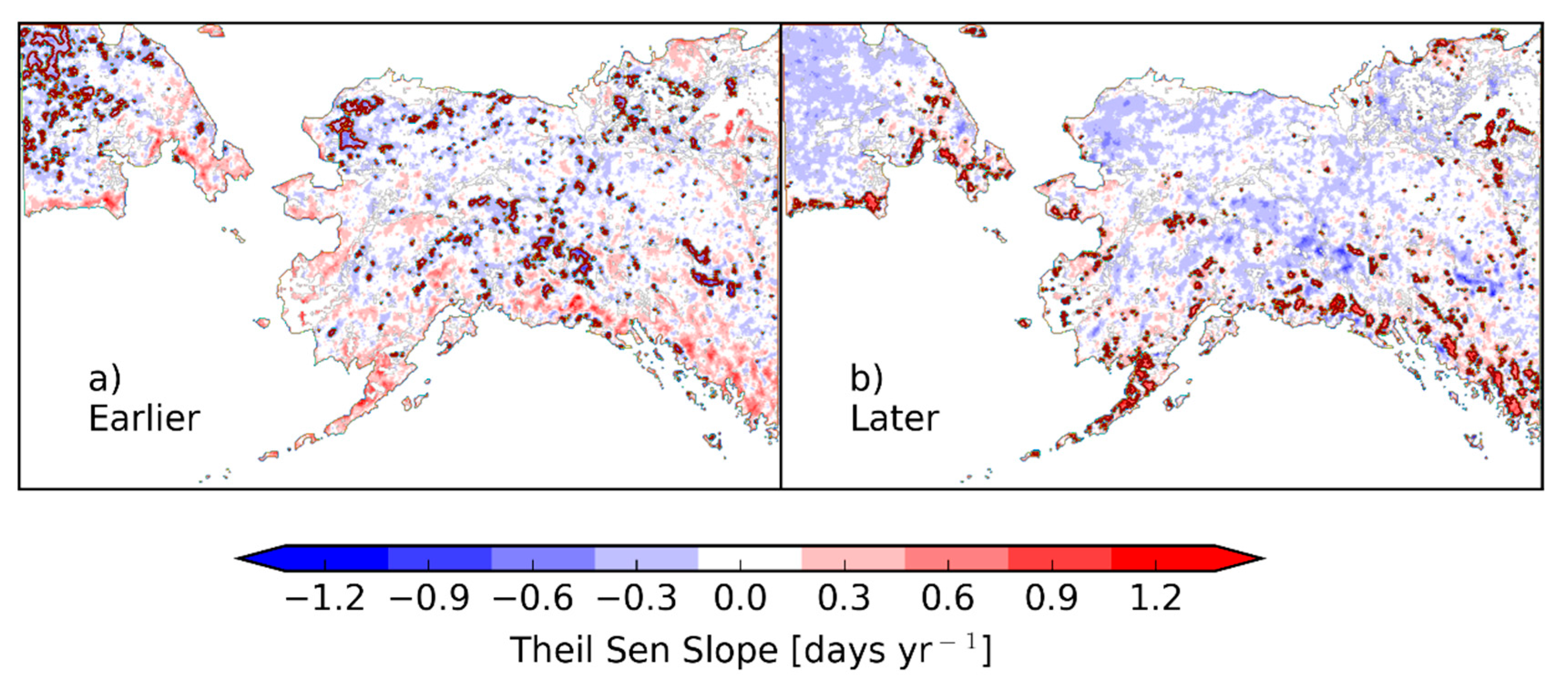
2.6. SO Trend Analysis
We performed temporal linear trend analysis for each grid cell to estimate the sign and strength of PMW SO changes over the satellite record (1988–2016). A Theil–Sen (TS) approach was used to compute the trend slope as the median value between each paired point [
59]. The TS is a robust trend estimation for non-parametric time-series that do not meet the assumptions for data normality and homoscedasticity, while also being resilient to outlier effects. Significant trends were identified using the Mann–Kendall Test (MKT) and were considered significant where
p < 0.1 [
60].
4. Discussion
The satellite PMW SO retrieval method and results described in this study performed well in relation to independent SO estimates derived from in situ SNOTEL station measurements across Alaska (r = 0.66−.92; MAE = 2–10 days). The PMW SO performance at these sites was also within ±10 days of other established geospatial SO records from the IMS, Landsat, and MODIS. These results are consistent with a prior study reporting similar PMW-derived SO accuracy over the European boreal-arctic [
30]. Residual differences between the PMW SO results and more established geospatial SO records were also within ±10 days across a majority (≥70%) of the entire Alaska domain, and below the 14–16 day estimated precision of the Landsat and MODIS derived SO products. Regional differences between the PMW SO retrievals and other SO benchmarks were attributed to the different sensitivity of optical and microwave frequencies to snow and other landscape features, as well as the different classification algorithms, spatial footprints and temporal fidelity of the observations used for the SO retrievals.
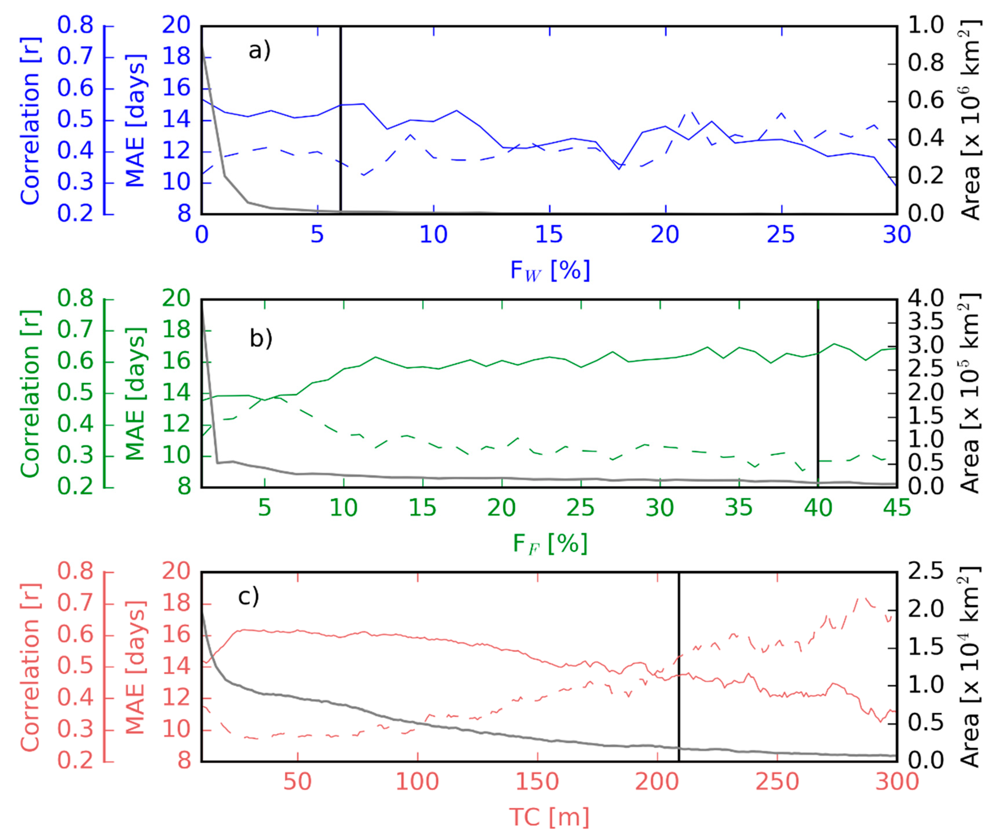
We examined the pattern of PMW SO relative errors in relation to selected landscape features expected to contribute to PMW uncertainty, including topographic complexity (TC), fractional water (FW), and forest cover (FF) within each 6.25 km resolution PMW grid cell. Our results indicate a general decline in PMW SO performance with increasing TC, defined as the spatial standard deviation of the elevation within a grid cell. These results are consistent with the coarser footprint PMW Tb retrievals being more constrained in their ability to characterize sub-grid scale SO heterogeneity in complex landscapes relative to the finer scale optical remote sensing observations. Nevertheless, the Tb product used for this study [
42,
65] provides a 2–4-fold spatial resolution enhancement over other available standard PMW products for the same Tb frequencies [
26,
57,
66], while preserving the benefit of near daily Tb temporal fidelity.
We found a smaller than expected FW influence on PMW SO uncertainty (e.g.,
Figure 8), despite surface water having a strong influence on microwave emissions [
56]. We attributed the lower-than-expected FW sensitivity to the screening of higher FW grid cells prior to the SO algorithm implementation, and the predominantly low FW cover of the remaining 6.25 km resolution Tb grid cells used for the SO classification. However, our results indicated greater FW cover (1% increase) during anomalous warm years relative to cool years over the domain, suggesting that the enhanced water may contribute to greater PMW SO uncertainty in warmer years. High springtime FW in Alaska may be attributed to flooding of low-lying areas enhanced by snow runoff generated during a short snowmelt period when the soil is still frozen [
67] and enhanced melting of permafrost [
68]. Variability in annual FW is largely a response of spatial heterogeneity in climate, surface topography and permafrost conditions, but is largely governed by seasonal temperatures in the Arctic [
69,
70].
Surprisingly, the PMW SO results were relatively robust to increasing FF cover and even indicated improved SO consistency at higher FF levels relative to the other benchmark observations. These results contrast with prior studies indicating elevated Tb levels over Alaska interior forest regions, relative to lower Tb values expected over snow covered areas [
71]. Given that the PMW SO algorithm is governed by the 19 and 37 GHz Tb difference, the expected elevation in Tb values and reduced Tb frequency gradient would be expected to reduce the effective GRP signal-to-noise ratio over dense forests [
46]. Forests are also expected to attenuate microwave emissions from surface snow cover [
72], further contributing to PMW SO uncertainty. The PMW record shows relatively early SO bias over much of the Alaska interior, which may reflect uncertainty contributed from the extensive forest cover in the region. The boreal forest structure tends to be closed [
73], which may contribute to a stronger signal from the underlying snowpack. A stronger-than-expected microwave snow signal, coupled with significant uncertainties from optical remote sensing of snow in forested regions [
21] may explain the apparent robust PMW SO response to FF.
Other factors may contribute to PMW SO uncertainty beyond the limited landscape attributes examined in this study. For example, a PMW tendency toward earlier SO timing in southwest Alaska relative to the other SO records may reflect generally shallow seasonal snow cover and tundra shrub conditions in this region, where a shallow snowpack (i.e., <5 cm depth or <10mm SWE) is largely transparent to PMW frequencies below 25 GHz [
23]; while the PMW frequencies used in this study are less sensitive to shallow snow cover, the corresponding snow signal is much stronger for optical sensing in the absence of potential degradation from overlying vegetation, low solar illumination or clouds. The PMW results indicated a general 5–10 day SO delay relative to the other geospatial SO records in colder climate areas, including the Arctic North Slope, Brooks, and Alaska Ranges. This difference is within the estimated uncertainty of the SO records from Landsat and MODIS, which may be further elevated by optical remote sensing retrieval errors under unfavorable conditions including persistent cloud cover. The MODIS LCLD has been noted to precede snow depth observations [
13] and is in agreement with our results showing generally early MODIS SO bias relative to the SNOTEL SO observations in the Alaska North Slope and Western regions. Both MODIS and Landsat may show similar SO uncertainty in the region because of extensive data loss from persistent cloud cover formed under orographic conditions in mountain landscapes [
74], as well as shadows created from topographic complexity [
75].
The PMW regional trend analysis indicated generally earlier SO conditions over approximately 51% of the domain, but with only 9% of the negative trend areas significant (
p < 0.1). These results are in general agreement with several studies showing a decline in snow cover extent and duration at higher latitudes [
8,
76,
77], but also more diverse and of lower magnitude than expected given the Arctic amplification and increasing temperatures [
3,
78]. Our PMW SO trends may be tempered by the purported
global warming hiatus which extended from 1998–2013 [
79,
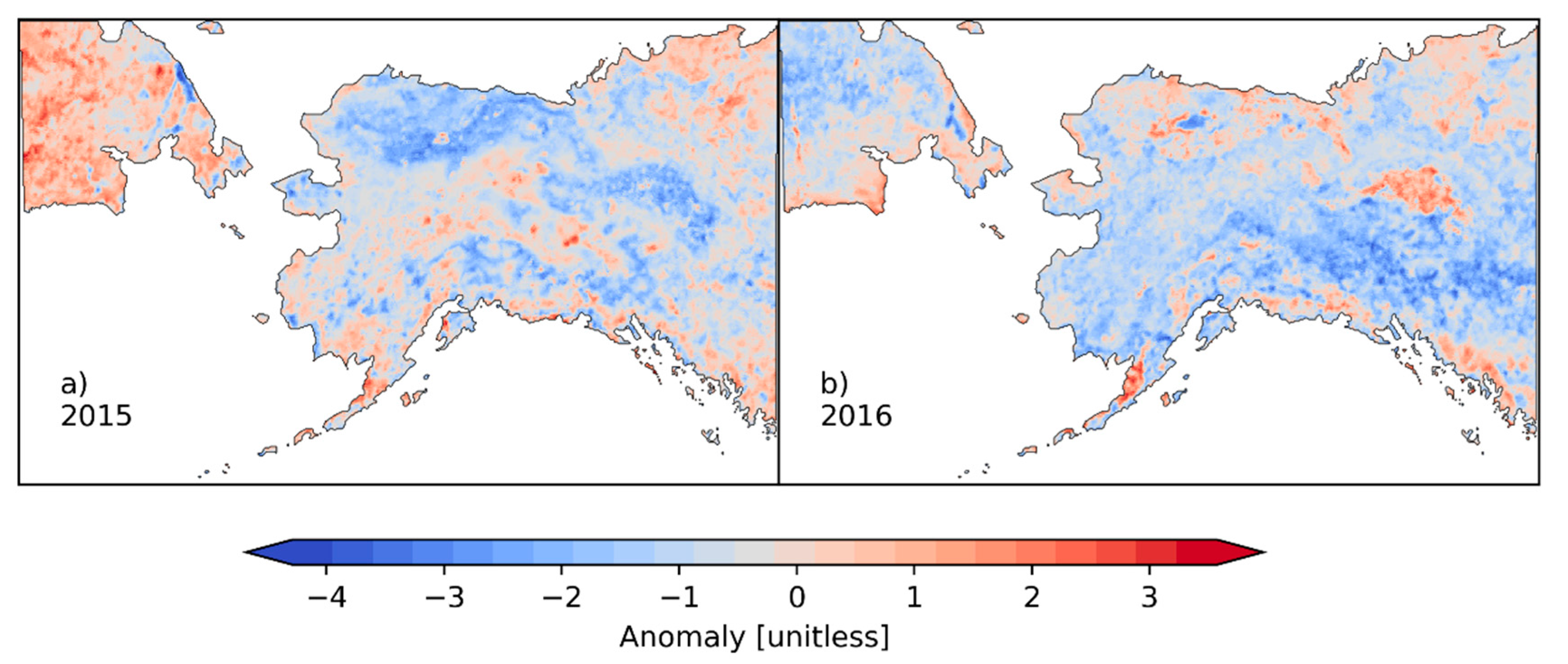
80]. The SO trends may also be influenced by the large characteristic regional climate variability superimposed on a smaller longer-term environmental trend, and represented by a limited 29-year satellite record. However, the observed annual SO anomalies generally coincide with documented warm and cool annual temperature anomalies in the region, as temperatures have been identified as a major driver of SO timing at lower elevations [
76]. As temperatures across the Arctic are projected to increase into the future [
3], greater variability in snow cover conditions, including SO date, are expected.
5. Summary and Conclusions
The SO date is an important governor of ecologic and hydrologic processes across Alaska and Arctic-Boreal landscapes, yet a better understanding of regional patterns and trends in SO timing has been limited by a regionally sparse in situ observation network and uncertainties in geospatial SO records derived from available satellite observations and models. Uncertainties in the geospatial SO records stem from multiple factors, including different retrieval methods with variable sensitivity, spatial resolution, timing and duration of observations. In this study, we presented a satellite PMW SO retrieval method that exploits the differential response between daily 19V and 37V GHz Tb channels with daily repeat and 6.25 km resolution gridding from 1988–2016 over Alaska. The resulting PMW SO data record compliments other satellite-based SO records derived from optical remote sensing, including MODIS [
13] and Landsat [
31], by exploiting the unique microwave sensitivity to snow cover while extending the SO record over a longer (29-year) period. The PMW SO retrievals benefit from daily satellite Tb observations at higher latitudes (>50°N), but with relatively coarse spatial gridding compared with optical remote sensing-based products with finer (30 m to 500 m) spatial resolution but much coarser temporal sampling and compositing of the underlying observations because of orbital geometry, illumination, and cloud-atmosphere constraints.
The PMW SO record showed favorable accuracy in relation to independent in situ SO observations from Alaska SNOTEL weather stations (r = 0.66–0.92; MAE = 2–10 days). The PMW accuracy at these sites was also consistent with the performance of other geospatial SO benchmarks obtained from the IMS, MODIS, and Landsat. Analysis of regression residuals between the PMW SO retrievals and other geospatial SO benchmarks indicated relative PMW SO consistency within ±10 days of the other SO records over an average 75% of the study domain, which was also within the estimated precision of the SO benchmark observations. The PMW retrievals tended to show delayed SO timing relative to the other geospatial SO records in colder tundra and mountain areas, including the North Slope, Brooks, and Alaska Ranges; however, the PMW SO timing was comparatively early over the Alaska interior and southwest. Regional differences in SO timing were attributed to the underlying PMW and optical sensor retrievals with different sampling footprints, varying sensitivity to snow properties and potential signal degradation from cloud-atmosphere effects, surface water, vegetation cover, and terrain complexity. Despite these differences, the PMW SO performance over the entire domain was within ±11 days of the other geospatial records, which was consistent with the in situ SNOTEL validation assessment and within the estimated precision of the SO benchmark observations.
A regional trend analysis of the 29-year PMW SO record indicated generally earlier SO timing across the domain, with a stronger tendency toward early SO conditions in anomalous warm years. Hence, as the high latitudes continue to warm, uncertainty remains in our understanding of how boreal-Arctic ecosystems and hydrological function will respond to earlier SO conditions. Our results also show snow cover persistence and SO delays in many areas, even during anomalous warm years, indicating potential resilience and refugia from climate change in the region. The global coverage and continuing operations of PMW satellites provide the means for potential monitoring of SO conditions across the pan boreal-Arctic domain. The continuity of these observations also spans multiple decades, enhancing capabilities for distinguishing relatively subtle SO trends from a background of large characteristic regional climate variability.


