Trends in High School Dropout and Completion Rates in the United States

Defining and Calculating Averaged Freshman Graduation Rates Using the CCD

National Center for Education Statistics (NCES) uses data from the Common Core of Data (CCD) to calculate averaged freshman graduation rates (AFGRs). The AFGR also uses CCD enrollment data collected through EDFacts data group 39 within file 052 as well as CCD graduate counts collected through EDFacts data group 306 within file 040. For more information about these data groups, please see file specifications 052 and 040 for the relevant school years, available at http://www2.ed.gov/about/inits/ed/edfacts/file-specifications.html

The AFGR provides an estimate of the percentage of high school students who graduate within 4 years of first starting 9th grade. The rate uses aggregate student enrollment data to estimate the size of an incoming freshman class and counts of the number of diplomas awarded 4 years later. The incoming freshman class size is estimated by summing the enrollments in 8th grade in year one, 9th grade in year two, and 10th grade in year three, and then dividing by three. The averaging has a smoothing effect that helps compensate for prior-year retentions in the 8th-, 9th-, and 10th-grade enrollment counts. Although not as accurate as a 4-year graduation rate computed from a cohort of students using student record data like the adjusted cohort graduation rate (ACGR), the AFGR can be computed with widely available cross-sectional data. Based on a technical review and analysis of several different 4-year graduation rates, the AFGR was selected as the most accurate indicator, excepting only the ACGR, from a number of alternative estimates that can be calculated using available crosssectional data (Seastrom et al. 2006a, 2006b). The following formula provides an example of how the AFGR would be calculated for the graduating class of 2012–13:¹

Number of regular high school diplomas awarded in SY 2012–13

(The number of 8th-graders enrolled in the fall of 2008 plus the number of 9th-graders enrolled in the fall of 2009 plus the number of 10th-graders enrolled in the fall of 2010) divided by 3

The AFGR was intended to address a lack of regular information about the timeliness of graduating from public high schools. Precise measures of how long it takes for a student to graduate high school require data sources that follow the progress of each individual student over time. Until recently, most states lacked data systems that captured individual public school studentlevel data over time. The AFGR was developed to utilize data that were available across the 50 states on a regular basis to provide a general and comparable measure of the percentage of public high school students who graduate with a regular high school diploma within 4 years of first entering 9th grade. The AFGR is useful for time series analyses of graduation rates, since the data used to generate the AFGR are available going back in time to at least the 1960s.

State and local policies can affect the number of regular high school diploma recipients reported. There are differences in what a regular high school diploma represents across states. The CCD collection defines a regular diploma as the high school completion credential awarded to students who meet or exceed coursework and performance standards set by the state or other approving authority. While this language provides a definition of common intent, the requirements to earn a high school diploma varies among states, including, for example, attendance requirements, coursework requirements, and exit exams.

Defining and Calculating Adjusted Cohort Graduation Rates

EDFacts 4-year ACGR data are collected in data group 695 within file 150 and in data group 696 within file 151. EDFacts collects these data groups on behalf of the Office of Elementary and Secondary Education. For more information about these data groups, please see file specifications 150 and 151 for the relevant school year, available at http://www2.ed.gov/about/inits/ed/edfacts/file-specifications.html.

The ACGR is calculated based on the number of students who graduate in 4 years or less with a regular high school diploma divided by the number of students who form the adjusted cohort for the graduating class. In order to calculate and report the 4-year ACGR, states must follow the progress of each individual 9th- to 12th-grade student over time and maintain documentation of students who enter or leave schools or districts within their state. From the beginning of 9th grade (or the earliest high school grade), students who are entering that grade for the first time form a cohort that is “adjusted” by adding any students who subsequently transfer into the cohort from another state and subtracting any students who subsequently transfer out, emigrate to another country, or die. The following formula provides an example of how the 4-year adjusted cohort is calculated.

The ACGR rate for the 2016–17 class is formulated as follows:

Number of cohort members who earned a
regular high school diploma by the end of SY 2016–17

Number of first-time 9th-graders in fall 2013 (starting cohort)
plus students who transferred in, minus students who
transferred out, emigrated, or died during school
years 2012–13, 2013–14, 2014–15, 2015–16, and 2016–17

State education agencies (SEAs) report ACGR data for each school and local education agency (LEA), and for the state total cohort rate. The methodology of the ACGR, as it was designed, allows for the movement or transfer of students from one school to another, while only counting each student once. A student may change schools and thus exit their prior school’s cohort and enter their new school’s cohort, but stay in the same district and state cohort. Similarly, a student who changes districts within a state will move to the new school and district cohort for the ACGR, but will stay in the state’s cohort. In order to subtract or transfer a student out of a cohort, the school or LEA must have official written documentation that the student enrolled in another school or in an educational program that culminates in the award of a regular high school diploma.

Unless specified, the ACGR data in this report and the associated data files reflect the data as reported by each SEA. The ACGRs required under the current Title I regulations are more comparable across states than were graduation rates submitted by SEAs under prior regulations. However, there has been some variation in the way that individual states have interpreted and understood the methodology specified in the statute. Examples of ways the calculated ACGR may vary among states include

• how students are identified for inclusion in certain subgroups;
• how the beginning of the cohort is defined;
• whether summer school graduates are counted as on-time graduates; and
• the criteria of what constitutes a diploma that meets the regulatory definition of a regular high school diploma.²

Defining and Calculating Dropout and Completion Rates Using the CPS

The Current Population Survey (CPS) is the only source of national time series data on dropout and completion rates. The CPS data are also good for studying correlations between educational outcomes and other important issues such as employment and earnings. However, because the CPS collects no information on school characteristics and experiences, its usefulness in addressing dropout and completion issues is primarily for providing insights on who drops out and who completes school. Sample sizes in the CPS collections do not support stable state-level estimates.

There are important differences in data collection procedures between the CPS and the CCD. First, the CCD collection includes only data for public schools, whereas the CPS counts include students who were enrolled in either public or private schools and some individuals who were never enrolled in school in the United States. Second, the CCD collects data about students from a given state’s public school system. CPS data are based on where individuals currently reside, so the state of residence may differ from the state or country of earlier school attendance. Third, the CCD collection is based on administrative records rather than on individual self-reports based on household surveys, as in the CPS. Finally, data in the CCD are collected from the full universe of public schools, whereas data in the CPS are collected from a sample of households, not the full universe of households. As a result, CPS data have sampling errors associated with estimates, whereas CCD data do not. For more information on CPS sampling errors and how to interpret them, see “Statistical Procedures for Analyzing CPS- and American Community Survey (ACS)-Based Estimates” on the following pages.

Defining and Calculating Dropout and Completion Rates Using the CPS

Event Dropout Rates

The October Supplement to the CPS is the only national data source that can currently be used to estimate annual national dropout rates. As a measure of recent dropout experiences, the event dropout rate measures the proportion of students who dropped out over a 1-year interval.

The numerator of the event dropout rate for 2016 is the number of persons ages 15–24³ surveyed in October of the current year who were enrolled in school⁴ in October of the previous year, who were not enrolled in high school or postsecondary education in October of the current year, and who did not complete high school (i.e., had not received a high school diploma or an alternative credential such as a GED) between October of the previous year and October of the current year.

The denominator of the event dropout rate is the sum of the dropouts (i.e., the numerator) and all persons ages 15–24 who were enrolled in school in October of the previous year⁴ and were either still enrolled in high school or postsecondary education in October of the current year or graduated or completed high school between October of the previous year and October of the current year.⁵

The dropout interval is defined to include the summer prior to the October CPS survey and the previous school year, so that once a grade is completed, the event dropout rate then measures whether the student completed the next grade. Given that the data collection is tied to each person’s enrollment status in October of two consecutive years, any student who drops out and returns within the 12-month period is not counted as a dropout.

Status Dropout Rates

The status dropout rate reflects the percentage of individuals who are dropouts, regardless of when they dropped out. The numerator of the status dropout rate for the current year is the number of individuals ages 16–24⁶ who, as of October of the current year, had not completed high school and were not currently enrolled. The denominator is the total number of 16- to 24-year-olds in October of the current year.

Status Completion Rates

The numerator of the high school status completion rate is the number of 18- to 24-year-olds⁷ who had received a high school diploma or an alternative credential such as a GED. The denominator is the number of 18- to 24-year-olds who are no longer in elementary or secondary school.

GED Credentials and the Status Completion Rate. Editions of this series of high school completion and dropout reports that were released prior to 2000 presented estimates of overall status completion rates and estimates of the method of completion— graduation by diploma or completion through an alternative credential such as the GED—based on data obtained through CPS reporting. Because of the changes that were introduced in the CPS in 2000, data on the method of completion for 2000 and later years were not comparable with data on the method of completion for years prior to 2000; in addition, pre-2000 CPS estimates and method-of-completion data were no longer reported in NCES reports generally. Please see the discussion of the GED Testing Service data below for further information.

Additional Considerations Regarding CPS Data

Over the last several decades, CPS data collection procedures, items, and data preparation processes have changed. Some of these changes were introduced to ensure that CPS estimates were comparable to those from decennial Census collections, some were introduced to reflect changes in the concepts under study, some were introduced to improve upon measures, and some were introduced to develop measures for new phenomena. The effects of the various changes have been studied to help ensure they do not disrupt trend data from the CPS. For a summary of the changes and studies of their effects, please see appendix C of Dropout Rates in the United States: 2001 (Kaufman, Alt, and Chapman 2004).

CPS data include weights to help make estimates from the data representative of the civilian, noninstitutionalized population in the United States. These weights are based on decennial Census data that are adjusted for births, deaths, immigration, emigration, etc., over time.

Imputation for Item Nonresponse in the CPS. For many key items in the October CPS, the U.S. Census Bureau imputes data for cases with missing data due to item nonresponse. However, the Census Bureau did not impute data regarding the method of high school completion before 1997. Special imputations were conducted for these items using a sequential hot-deck procedure implemented through the PROC IMPUTE computer program developed by the American Institutes for Research. The hot-deck method assigns imputed values from survey respondents who answered an item (donors) to similar survey respondents who did not (recipients). Donors and recipients are matched based on various respondent characteristics. For the CPS data, three categories of age, two categories of race, two categories of sex, and two categories of citizenship were used to match donors with recipients for any given item. The procedure ensures that information from one donor is not used for a large number of recipients. This prevents bias from being introduced into the dataset if all the recipients were imputed from one donor.

Age and Grade Ranges in CPS Estimates. The age and grade ranges used in the CPS measures of dropout rates are constrained by available data. Ideally, the estimates would be able to capture reliable estimates of children in grades as low as grade 9. However, the CPS asks the question about enrollment in the previous October only in terms of individuals age 15 and older. Many 9th-graders are younger than age 15, so 10th grade was selected as the lower boundary of grade ranges in the event dropout rate.

Accuracy of CPS Estimates. CPS estimates in this report are derived from samples and are subject to two broad classes of error—sampling and nonsampling error. Sampling errors occur because the data are collected from a sample of a population rather than from the entire population. Estimates based on a sample will differ to some degree (dependent largely on sample size and coverage) from the values that would have been obtained from a universe survey using the same instruments, instructions, and procedures. Nonsampling errors come from a variety of sources and affect all types of surveys—universe as well as sample surveys. Examples of sources of nonsampling error include design, reporting, and processing errors and errors due to nonresponse. The effects of nonsampling errors are more difficult to evaluate than those that result from sampling variability. To the extent possible, procedures are built into surveys in order to minimize nonsampling errors.

The standard error is a measure of the variability due to sampling when estimating a parameter. It indicates how much variance there is in the population of possible estimates of a parameter for a given sample size. Standard errors can be used as a measure of the precision expected from a particular sample. The probability that a sample statistic would differ from a population parameter by less than the standard error is about 68 percent. The chances that the difference would be less than 1.65 times the standard error are about 90 out of 100, and the chances that the difference would be less than 1.96 times the standard error are about 95 out of 100.

Prior to 2010, standard errors for percentages and numbers of persons based on CPS data were calculated using the following formulas:

Percentage:

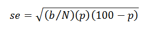
where p = the percentage (0 < p < 100),
N = the population on which the percentage is based, and
b = the regression parameter, which is based on a generalized variance formula and is associated with the characteristic.

Number of persons:

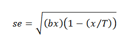
where x = the number of persons (i.e., dropouts),
T = population in the category (e.g., Black 16- to 24-year-olds), and
b = as above.

For instance, in 2009, b is equal to 2,131 for the total and White population, 2,410 for the Black population, 2,744 for the Hispanic population, and 2,410 for the Asian/Pacific Islander population ages 14–24. For regional estimates, b is equal to 1.06 for the Northeast, 1.06 for the Midwest, 1.07 for the South, and 1.02 for the West.

CPS documentation explains the purpose and process for the generalized variance parameter:

Experience has shown that certain groups of estimates have similar relations between their variances and expected values. Modeling or generalizing may provide more stable variance estimates by taking advantage of these similarities. The generalized variance function is a simple model that expresses the variance as a function of the expected value of a survey estimate. The parameters of the generalized variance function are estimated using direct replicate variances. (Cahoon 2005, p. 7)

Beginning with the 2010 CPS data, standard errors were estimated using Fay’s Balanced Repeated Replication (Fay-BRR). While the generalized variance model provides an estimate for standard errors, BRR better accounts for the two-stage stratified sampling process of the CPS, where the first stage of the CPS Primary Sampling Unit is the geographic area, such as a metropolitan area, county, or group of counties. The second stage is households within these geographic areas. For the CPS October supplement, 160 replicate weights were used in Fay-BRR calculations.

American Community Survey Data Considerations

Estimates from the ACS in this report focus on status dropout rates for the institutionalized population and for the noninstitutionalized population. The rates are derived using the same approach as that used for estimating status dropout rates from the CPS data. ACS data include weights to make estimates from the data representative of households and individuals in the United States. These weights are based on annual population updates generated by the Census Bureau to be representative of the U.S. population as of July 1. Data are fully imputed before release to the public, and flags are available to identify which values have been imputed for which cases.

Replicate weights that account for the complex sample design of the ACS have been developed for use in deriving variance estimates. Variance estimates for any full-sample ACS survey estimate are calculated using the following formula:

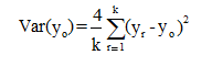
Where:
r = The replicate sample (r = 1......k)
o = The full sample
k = The total number of replicate samples (k = 80)
y_o = The survey estimate using the full-sample weights
y_r = The survey estimate using the replicate weights from replicate r

This variance estimate is the product of a constant and the sum of squared differences between each replicate survey estimate and the full-sample survey estimate.

The estimates and standard errors based on ACS data in this report were produced in SAS using the jackknife 1 (JK1) option as a replication procedure. The multiplier was set at 0.05 (4/80=0.05). Eighty replicate weights, PWGTP1 to PWGTP80, were used to compute the sampling errors of estimates.

Statistical Procedures for Analyzing CPS- and ACS-Based Estimates

Because CPS and ACS data are collected from samples of the population, statistical tests are employed to measure differences between estimates to help ensure they are taking into account possible sampling error.⁸ The descriptive comparisons in this report were tested using Student’s t statistic. Differences between estimates are tested against the probability of a type I error,⁹ or significance level. The significance levels were determined by calculating the Student’s t values for the differences between each pair of means or proportions and comparing these with published tables of significance levels for two-tailed hypothesis testing.

Student’s t values may be computed to test the difference between percentages with the following formula:

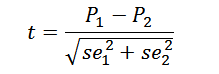
where P₁ and P₂ are the estimates to be compared and se₁ and se₂ are their corresponding standard errors.

Several points should be considered when interpreting t statistics. First, comparisons based on large t statistics may appear to merit special attention. This can be misleading since the magnitude of the t statistic is related not only to the observed differences in means or proportions but also to the number of respondents in the specific categories used for comparison. Hence, a small difference compared across a large number of respondents would produce a large t statistic.

Second, there is a possibility that one can report a “false positive,” or type I error. In the case of a t statistic, this false positive would result when a difference measured with a particular sample showed a statistically significant difference when there was no difference in the underlying population. Statistical tests are designed to control this type of error. These tests are set to different levels of tolerance or risk, known as alphas. The alpha level of .05 selected for findings in this report indicates that a difference of a certain magnitude or larger would be produced no more than 1 time out of 20 when there was no actual difference between the quantities in the underlying population. When p values are smaller than the .05 level, the null hypothesis that there is no difference between the two quantities is rejected. Finding no difference, however, does not necessarily imply that the values are the same or equivalent.

Third, the probability of a type I error increases with the number of comparisons being made. Bonferroni adjustments are sometimes used to correct for this problem. Bonferroni adjustments do this by reducing the alpha level for each individual test in proportion to the number of tests being done. However, while Bonferroni adjustments help avoid type I errors, they increase the chance of making type II errors. Type II errors occur when there actually is a difference present in a population, but a statistical test applied to estimates from a sample indicates that no difference exists. Prior to the 2001 report in this series, Bonferroni adjustments were employed. Because of changes in NCES reporting standards, Bonferroni adjustments are not employed in this report.

Regression analysis was used to test for trends across age groups and over time. Regression analysis assesses the degree to which one variable (the dependent variable) is related to one or more other variables (the independent variables). The estimation procedure most commonly used in regression analysis is ordinary least squares (OLS). When studying changes in rates over time, the rates were used as dependent measures in the regressions, with a variable representing time and a dummy variable controlling for changes in the educational attainment item in the current year
(= 0 for years from 1 to 40 years before the current year, = 1 for years after the current year) used as independent variables. Significant and positive slope coefficients suggest that rates increased over time. Conversely, significant and negative coefficients suggest that rates decreased over time. Because of varying sample sizes over time, some of the estimates were less reliable than others (i.e., standard errors for some years were larger than those for other years). In such cases, OLS estimation procedures do not apply, and it is necessary to modify the regression procedures to obtain unbiased regression parameters. This is accomplished by using weighted least squares regressions.¹⁰ Each variable in the analysis was transformed by dividing by the standard error of the relevant year’s rate. The new dependent variable was then regressed on the new time variable, a variable for 1 divided by the standard error for the year’s rate, and the new editing-change dummy variable. All statements about trend changes in this report are statistically significant at the .05 level.

¹ Eighth-, 9th-, and 10th-grade enrollments were adjusted to include a prorated number of ungraded students using the ratio of the specified grade enrollment to the total graded enrollment. The same ratio was used to prorate ungraded students for the disaggregated enrollment counts (race/ethnicity and gender).
² Under 34 C.F.R. § 200.19(b)(1)(iv), a regular high school diploma is defined as “the standard high school diploma that is awarded to students in the State and that is fully aligned with the State’s academic content standards or a higher diploma and does not include a high school equivalency credential, certificate of attendance, or any alternative award.”
³ This age range was chosen in an effort to include as many students in grades 10 through 12 as possible. Because the rate is based on retrospective data, it lags 1 year, meaning that some 15-year-olds have turned age 16 by the time of the interview.
⁴ Due to data limitations, grade 9 event dropouts could not be reliably calculated, so the calculation of the event dropout rate is restricted to grades 10–12. The current calculation potentially includes persons who were enrolled in grade 9 in October of the previous year and dropped out after completing grade 9.
⁵ Due to data limitations, this excludes persons who were enrolled in grade 10 in October of the previous year and who were still enrolled in grade 10 in October of the current year, as well as persons who graduated or completed high school between October and December of the previous year.
⁶ Age 16 was chosen as the lower age limit because, in some states, compulsory education is not required after age 16. Age 24 was chosen as the upper limit because it is the age at which free secondary education is no longer available and the age at which the average person who is going to obtain a GED does so.
⁷ Age 18 was chosen as the lower age limit because most diploma holders earn their diploma by this age. Age 24 was chosen as the upper limit because it is the age at which free secondary education is no longer available and the age at which the average person who is going to obtain a GED does so.
⁸ Data from the CCD are from universe data collections and therefore do not require statistical testing such as that used for estimates from the CPS sample survey data.
⁹ A type I error occurs when one concludes that a difference observed in a sample reflects a true difference in the population from which the sample was drawn, when no such difference is present. It is sometimes referred to as a “false positive.”
¹⁰ For general discussion of weighted least squares analysis, please see Gujarati (1998).

Back to Top